Policy Optimization Methods in Reinforcement Learning
published 2026-02-12·created 2026-02-09·updated 2026-09-19
Overview
Unliked value-based methods, policy optimization methods search over policy parameters \(\theta\)directly in order to find parameters that maximize (or minimize) a policy objective function. They do not inherently need to exploit structured value representations for states (or state-action pairs) which are needed in value-based methods to compute an optimal policy; however, we will actually also see that modern policy optimization methods PPO/TRPO/A3C/SAC actually still learn \(V_{\phi}(s)\) or \(Q_{\phi}(s,a)\) as baselines in practice to boost the efficacy of the base algorithm.
In the overall Taxonomy for Policy Optimization Methods, we roughly group these into 3 general methods
Evolutionary Methods: CEM, CMA-ES, NES
Biologically inspired methods that directly update policies through a selecting candidate \(\theta\) based on the survival of the fittest test on different policy parameters.
Policy Gradient Methods: REINFORCE
They optimize the parameters \(\theta\) directly by computing a gradient \(\frac{d}{d\theta}\) of a policy function - typically an estimate - \(U(\theta)\) and optimizing them via gradient ascent.
Actor-Critic Methods: A2C/A3C, PPO, SAC
A variant of policy gradient methods that introduce value functions \(V_{\phi}(s)\) or \(Q_{\phi}(s,a)\) (critics) for more stable updates of our policy (actor)
In comparison to value-based methods, policy-based methods are
5. more effective in high-dimensional + continuous action spaces
Value-based methods select optimal actions based on something like \(\arg \max_{a} Q(s,a)\) that isn’t feasible across high dimensions.
6. stochastic
Policy-based methods typically are stochastic: this is because our policy parameters \(\theta\) parameterize a distribution that our actions are sampled from. Remember that value-based methods need to rely on heuristics like epsilon-greedy to embed exploration in their policies.
Why is stochasticity a good thing?
- exploration is optimal to train any policy
- in partial-observability settings/environments, deterministic mappings aren't the optimal solution
I. Evolutionary Methods for Policy Search
Evolutionary Methods in Reinforcement Learning
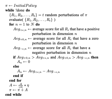
Evolutionary Search as Black-Box Policy Optimization
These are called evolutionary methods because they closely follow the evolution of a population!
Initialize a population of policy parameter vectors \(\theta_{i}\) randomly
aka Genotypes
Make random perturbations to each parameter vector \(\theta_{i}'\)
Simulating mutations in offspring
Evaluate the perturbed parameter vector along some fitness function \(F(\theta_{i}')\)
Survival of the fittest
Update your policy parameters to favor the best performing parameter vectors based on fitness score \(F(\theta)\)
Enabling fitness in this offspring
These are examples of black-box policy optimization, where we treat the policy and environment as a “black box” that we can query (run rollouts) and update our policy based purely on performance we can observe
we do not learned a structured “state” representation of state values and/or state-action values based on the structure of Bellman equations like in Value-Based Methods in Reinforcement Learning
use do not use analytic gradients of the return w.r.t. policy parameter \(\theta\) directly (as in Policy Gradient Methods in Reinforcement Learning). Methods like NES may do so indirectly, where we compute gradients w.r.t the parameters \(\phi\) of a search distribution that \(\theta\) is drawn from. There is subtle, but huge difference!
CEM: Cross-Entropy Method
In this method we consider policy parameters sampled from a isotropic Gaussian matrix:
Initialize a search distribution \(p_{\phi}(\theta)\) where \(\mu=0\) and \(\Sigma = 100I\)
Repeat for \(k\) steps:
sample \(n\) policy parameters \(\{ \theta_{i} \}_{i=1}^n\) from current multivariate Gaussian distribution matrix
Evaluate those \(n\) parameters averaged over \(L\) rollouts to generate a reward signal or scalar return \(F(\theta_{i})\)
select a proportion \(\rho\) of those parameters with highest score as our \(\lfloor \rho n \rfloor\)elite samples!
use their corresponding \(\mu\) and \(\sigma^2\) to update our reference matrix for sampling, which basically means setting the new mean as the mean of those highest \(\lfloor \rho n \rfloor\) parameters and setting the new variance as simply the variance of those selected elite samples!
\[\begin{align} \\
& \mu \in \mathbb{R}^k ,\forall j \in [k]\\
& \mu(j) = \frac{1}{\lfloor \rho n \rfloor}\sum_{i=1}^{\lfloor \rho n \rfloor}\theta'_i(j) \\
& \sigma^2(j) = \frac{1}{\lfloor \rho n \rfloor}\sum_{i=1}^{\lfloor \rho n \rfloor} (\theta'_i(j) - \mu(j))^2 + \eta
\end{align}\]
This worked really well up to the 2010’s and in low dimensional search space dimensions, shown to work well in Tetris (Szita, 2006), where we can craft a value function that is a linear combination of 22 basis functions \(\phi(s)\) (individual column heights, height differences, etc)
\[V_{w}(s) = \sum_{i=1}^{22} w_{i} \phi_{i}(s)\]
and execute CEM on the weight vector \(w\), evaluating fitness score based on the mean reward that weight matrix gives when computing a policy based on \(V_{w}(s)\)!
These evolutionary search methods weren’t a threat to DQN implementations at the time because they couldn’t scale to large non-linear neural nets with thousands of parameters. The fact that we rely on random sampling to somehow perturb each dimension of the weights to the optimal direction isn’t really sample-inefficient in very high dimensions - what if \(w \in \mathbb{R}^{10^{9}}\)?
Variants like CMA-ES, NES, and OpenAI’s scalable ES method make iterative improvements on CEM - but there is a reason why modern policy optimization methods use the information of a gradient vector in order to realize the best policy as we will see in policy gradient methods later on.
CMA-ES: Covariance Matrix Adaptation
Instead of limiting ourselves to diagonal Gaussian, we search by learning a full covariance matrix so instead of just updating the mean and variances, we’re updating the entire matrix.
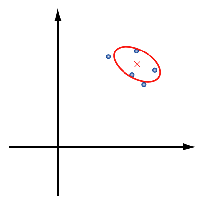
Imagine our samples are in 2-D dimension. Then visually, if there is an objective function we are trying to reach that is best maximized with samples spread in the shape 2d rotated ellipse, then we should utilize all the entries in a full covariance matrix which rotates a standard diagonal gaussian matrix (x-y aligned ellipse) to best maximize this objective function efficiently.
Our mean update can also be either a) iterative - as a weighted step from \(\mu_{t}\) towards the elites or b) a simple weighted recombination of the elites
Our covariance update now updates the covariance of the Gaussian search distribution to match the spread and correlations of the current elite set! We add a regularizer to prevent the variance from prematurely collapsing to \(0\) too quickly
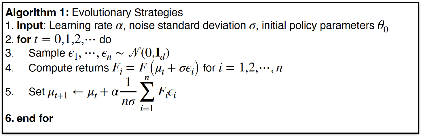
NES optimizes our expected fitness objective by updating the parameters of our search distribution through a natural gradient, specifically updating our learned mean \(\mu\), while fixing our covariance this time. NES considers every offspring when updating our policy parameters, because when deriving this gradient, we get an expectation term that has to be approximated with Monte-Carlo sampling.
Consider the parameters of our policy \(\theta \in \mathbb{R}^d\) are sampled from a Gaussian distribution with learned mean \(\mu \in \mathbb{R}^d\) and fixed diagonal covariance matrix \(\sigma^2I\) (which is not being learned). We denote this search distribution as \(P_{\mu}(\theta)\)
We really need to justify the intuition for why we use the log-probability trick: The point is we need to estimate the gradient using Monte-Carlo sampling, but to do that we need the pdf within the integral to convert to an expectation - when otherwise we just have \(\nabla_{\mu}P_{\mu}(\theta)\) !
To expand on that last step, in order to back propagate through Gaussian distributions to \(\mu\), then the sampling of \(\theta_{i} \sim \mathcal{N}(\mu, \sigma^2 I)\) needs to be converted through the reparameterization trick so that \(\theta_{i} = \mu + \sigma \epsilon_{i},\ \epsilon_{i} \sim \mathcal{N}(0, I)\).
From this derivation, we have shown that this gradient to update the mean \(\mu\) can be estimated by
sampling \(N\) parameters \(\theta_{i}\), running trajectories for each parameter, and obtaining our scalar fitness score \(F(\theta_{i})\) for each sample
Then we simply need to scale by a sampled noise term \(\epsilon\) divided by our variance \(\sigma\) and average out all scaled terms!
Based on this derivation we can now apply gradient ascent to iteratively update our \(\mu\)! (based on learning rate \(\alpha\))
We do not need to know anything about how we are computing our fitness score, we simply realize raw output returns given our samples \(\theta_{i}\)
We are not computing computing analytic gradients of \(F(\theta)\) wrt to \(\theta\) in order to update our policy parameters directly; in fact, we compute gradients wrt to a different, known object that we have set: the search distribution probability density \(P_{\mu}(\theta)\)
Scalability + Parallelization of ES
!REVISIT
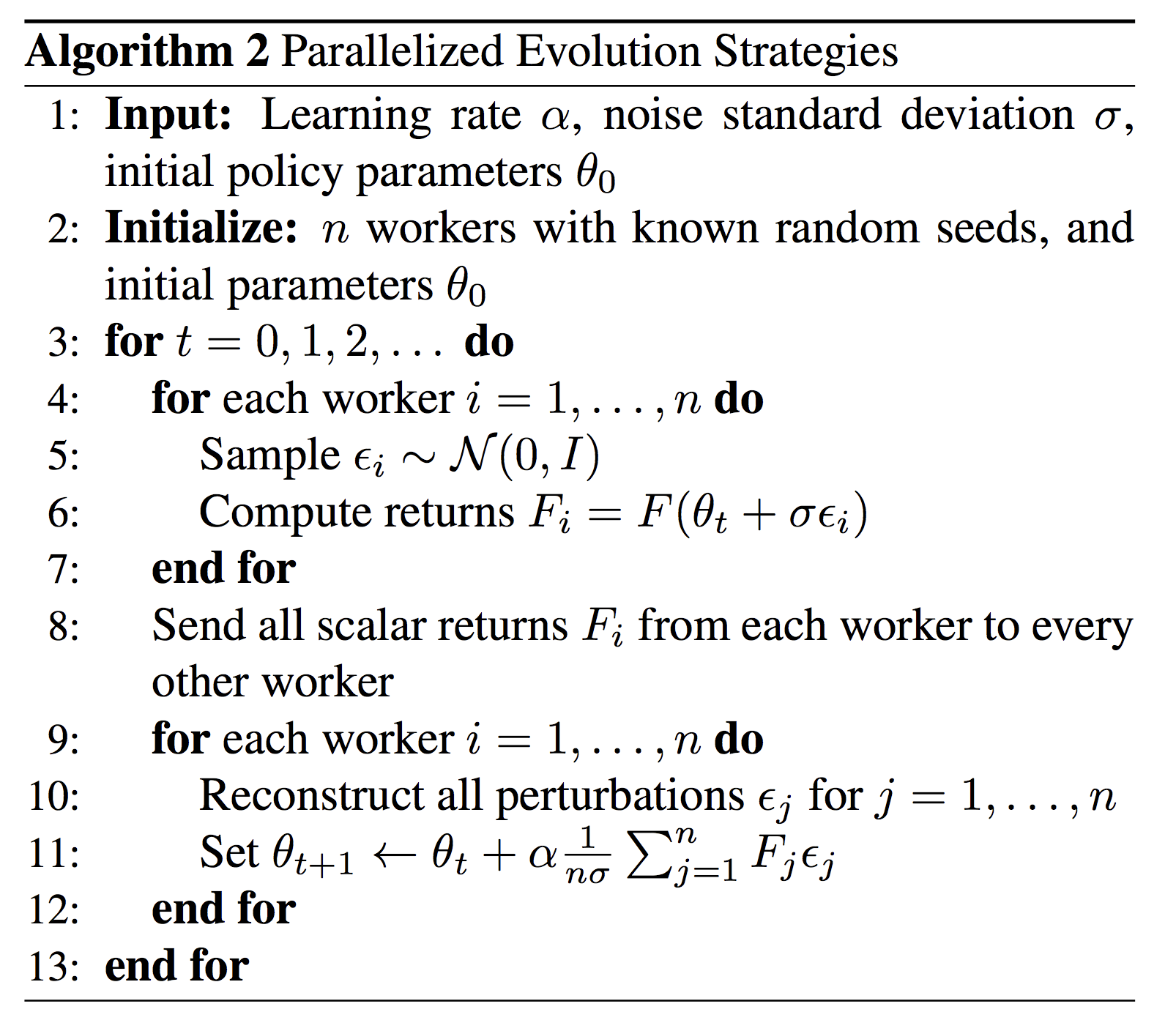
The reason why we can scale NES well for large dimension of policy parameters \(\theta\) when we are working with large policy networks is that we can parallelize the fitness score for each sampled \(\theta_{i}\) for a corresponding worker process, where each worker can individually compute this term \(\epsilon_{i} F_{i}(\theta_{i})\).
A bottleneck however, would be naively sending back and forth this large \(\theta_{i} = \mu_{t} + \sigma \epsilon_{i}\) vector across all our \(n\) workers:
Coordinator broadcasts \(\mu_{t}\) once per update step to all workers
Coordinator sends \(\epsilon_{i}\) to all \(n\) workers individually, which allows every worker to compute \(\theta_{i}\)
Each workers runs trajectories and sends back \(F(\theta_{i})\) to every other worker
Because of reparameterization only this \(\epsilon_{i}\) needs to be sent to all \(n\) workers, but this is still a very large parameter, so instead in a 2017 OpenAI paper, we use a pseudo random number generator to compute \(n\) (tiny) seeds and then send these known small seeds to the \(n\) workers, which can they reconstruct each large dimension \(\epsilon_{i}\) and compute our returns \(F(\theta_{i})\) which is just a scalar! So communication time is cut a lot.
(Salimans, Ho, Chen, Sutskever, 2017)
Note that here the current policy parameters \(\theta_{t}\) are the center/mean of the perturbation distribution \(\mu_{t}\)
Local Maxima Issue
ES methods can easily get stuck in local optima.
In order to prevent ES methods from getting stuck in local optima, we average fitness scores across
multiple tasks
related environments
so that the search is biased towards policy parameters that are robust to variations of task/environment similar the original set and not exploit local maxima in the original task/environment.
We no longer consider black-box optimization methods. Instead of updating a search distribution \(P(\theta)\) that our policy parameters are sampled from, we directly update our policy parameters \(\theta\), using gradient estimates computed from sampled trajectories (policy gradients)! Then we search for a local maximum of a policy objective \(U(\theta)\) by using gradient ascent.
Policy Objective
One reasonable policy objective is to maximize our expected trajectory reward over distribution of all trajectories parametrized by our policy parameters \(\theta\) .
Remember that \(P_{\theta}(\tau)\) is the probability distribution over seeing that entire trajectory when we run \(\pi_{\theta}\) in our environment which abstracts three key ingredients
the initial state being sampled from an initial state distribution
the dynamics of the environment resulting in stochastic next states \(s_{t+1}\)
the stochasticity of the policy in which actions are sampled from - this is what our \(\theta\) actually parameterizes.
It’s assumed that \(P_{\theta}(\tau)\) is a probability density function that is continuous and differentiable - necessary to propagate our gradient as we will see in the derivation: This really just means \(\pi_\theta(a\mid s)\) is a policy that is differentiable.
Overview
Then the general structure of Policy Gradient Methods would follow something like
Initialize policy parameters \(\theta\)
Sample trajectories \(\tau_{i} = \{ s_{t}^i, a_{t}^i \}_{t=0}^T\) by deploying the current policy \(\pi_{\theta}(a_{t}\mid s_{t})\)
Compute gradient vector \(\nabla_{\theta} U(\theta)\)
This is done through estimation from collected trajectories.
We now need to figure out how to compute this gradient in order to find optimal \(\theta\):
Aside: Finite-Difference Methods
One way to try and approximate policy gradient of \(\nabla_\theta U(\theta)\) by nudging \(\theta\) in every possible small amount dimension and approximate partial derivatives as such:
For each dimension \(k \in [n]\) calculate the partial gradient
In comparison to evolutionary methods, here the challenge is to compute derivatives w.r.t variables that parameterize a distribution that our expectation is summed over. The derivation uses the same log probability trick as derived for evolutionary methods; also we assume discrete trajectory space to sum over - if continuous, the derivation is largely the same.
The intuition is that our policy objective gradient is trying to
increase the log probability of trajectories that give a positive reward and
decrease the log probability of trajectories that give a negative reward.
The key observation is that this expectation can be simplified much further because our trajectories encapsulate the dynamics of the environment - but this is not specifically parametrized by our policy parameters, so the derivatives of our trajectories propagate further to specifically the derivatives of taking actions under our policy.
Given this estimate, let’s try to interpret more this gradient estimate \(\hat{g}\) is doing. During gradient ascent we update policy using \(\theta \leftarrow \theta + \alpha \hat{g}\) . So along some sampled trajectory \(\tau\) of all \(N\) trajectories we have that
If \(R(\tau)\) is high, then \(\hat{g}\) is updating the policy \(\theta\) to increase log-prob of taken action if it led to good return
(because we move in the direction \(\nabla_{\theta} \log \pi_{\theta}(a_{t}\mid s_{t})\)
If \(R(\tau)\) is bad along \(\tau\), then \(\hat{g}\) is updating the policy \(\theta\) to decrease log-prob of taken action if it led to bad return
Computing Policy Gradient
And the natural question is whether the derivative term is computable - which yes it is.
If our action space is continuous, then our policy network can be gaussian, outputting a mean and standard deviation. If we want our policy to be deterministic, then the action would be simply the mean!
So for multivariate gaussians (and for simplicity assume we are in the case where \(\Sigma\) is fixed), then
where we can back propagate \(\nabla_\theta \mu_\theta(s)\) through the mean part of the policy network.
What this looks like is:
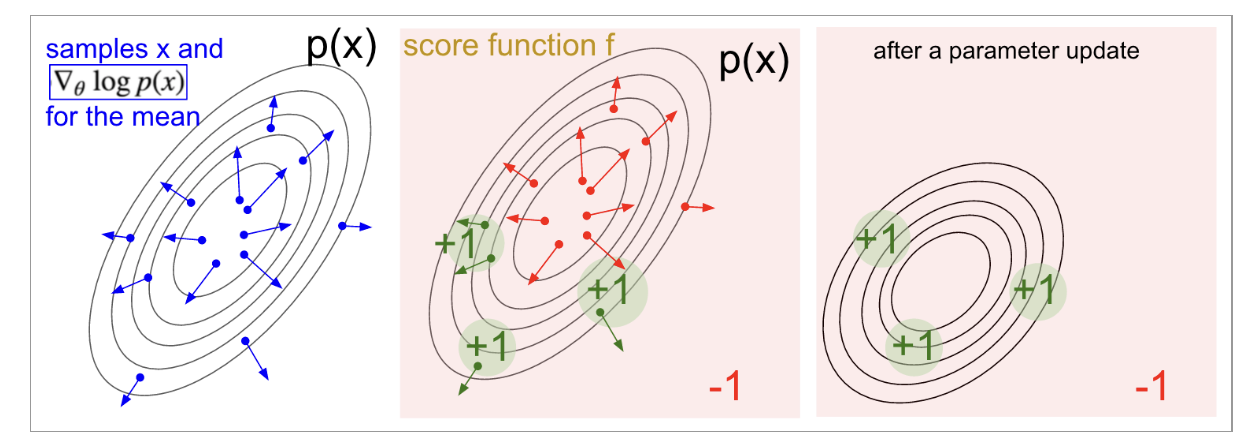
Blue points are samples from the current Gaussian centered at \(\mu\)
Each sample contributes a vector \(\Sigma^{-1}(x^{(i)}-\mu)\) (points outward from the mean, scaled/rotated by \(\Sigma^{-1}\))
high-reward samples pull the mean toward themselves; low-reward samples push it away!
Summing these gives an update direction that shifts \(\mu\) to \(\mu'\) favoring these high-reward actions
If our action space is discrete, obviously we apply a final softmax layer to output a discrete probability distribution over finite action space. Then if we want our policy to be stochastic, we can query a categorial distribution based on these probabilities for sampling.
If we go through the derivation, in simple terms the update is “increase the logit of the chosen action” minus “the weighted averaged logit gradient under the current policy” which is as follows:
Can we do better than assigning the standard cumulative trajectory reward \(R(\tau)\) for every action when computing gradient update? The issue with scalar \(R(\tau)\) is why should the action an agent takes at time step \(t\) be scaled by the reward trajectory of time steps that occurred before that \([0, t-1]\)?
Instead, we should emphasize causality: Only future rewards should be attributed to the action taken at time step \(t\) and each action takes the blame for the trajectory that comes after it:
One issue with weighting our gradient updates with \(G_{t}\) is the following situation:
a state \(s_1\) has all actions from here on out averaging out to a high positive magnitude reward of \(4000\)
a state \(s_{2}\) has all actions from here on out averaging out to a negative reward of \(-4000\)
Then no matter if we take a very bad action at \(s_1\) versus a very good action at state \(s_2\) the state’s baseline level of reward (expectation) is the major scaling factor in our gradient update, not the intention of whether we took a good or bad action in the first place. This is a huge mistake, our gradient updates should be weighted solely by how well this action does relative to other actions at this state, not by how good this state is relative to other states.
To counteract this we should then only consider the trajectory reward above our a fixed baseline (constant, time-dependent, or state-dependent) - which we call Advantages - at that state!
But how does this affect our policy objective estimate \(\hat{g}\)?
Actually, this new \(\hat{g}'\) is still unbiased estimator - it has the same expectation as our original \(\hat{g}\) - for our policy objective, because in expectation the baseline term has zero expectation, as long as \(b\) does not depend on the action \(a_{t}\). This means subtracting a baseline does not affect the convergence or efficacy of our gradient ascent updates!
It’s a bit easier to see first for constant baselines \(b\). The proof is easy here
\[\begin{align*}
\mathbb{E}_{\tau \sim P_{\theta}(\tau)}[\nabla _{\theta} \log P_{\theta}(\tau) b ] &= b \sum_{\tau} P_{\theta}(\tau) \nabla_{\theta} \log P_{\theta}(\tau)\\
&= b \sum_{\tau} \frac{P_{\theta}(\tau) \nabla_{\theta} P_{\theta}(\tau)}{P_{\theta}(\tau)} \\
&= b \cdot \nabla_{\theta} \sum_{\tau} P_{\theta}(\tau)= b \cdot \nabla_{\theta}[1] = 0
\end{align*}\]
But what if we have state-dependent baselines? Then if we zoom on a single time-step and condition our expectation on \(s_{t}\)
And our subtraction of baseline to consider relative reward has effectively reduced the scale of gradient updates \(\hat{g}\) quite a bit, thus we minimize variance overall!
Constant Baselines using the average return of the policy \(b = \mathbb{E}[R(\tau)]\)
Time-dependent Baselines\(b_t \approx \frac{1}{N}\sum_{i=1}^N G_t^{(i)}.\) where we average temporal reward over all trajectories
State-dependent Baselines
value function \(b(s_{t}) = V_{\pi}(s)\)
REINFORCE with BASELINE
The above discussion concludes REINFORCE with a state-dependent baseline, the Monte Carlo (likelihood-ratio) policy gradient method with variance reduction via a value function as baseline! We can still use other baselines but this is a common choice!
Initialize policy parameters \(\theta\) and baseline parameters \(\phi\) (value function \(V_\phi(s)\)).
Sample trajectories \(\{\tau_{i} = \{(s_{t}^{(i)}, a_{t}^{(i)})\}_{t=0}^{T-1}\}\) by deploying the current policy \(\pi_{\theta}(a_{t} \mid s_{t})\).
Compute returns \(G_t^{(i)} = \sum_{k=t}^{T-1}\gamma^{k-t} r(s_k^{(i)},a_k^{(i)})\) for all \(i,t\)
Fit the baseline \(V_\phi\) to the returns (by regression on \((s_t^{(i)}, G_t^{(i)})\).
Actor-Critic methods build off even further from our state-dependent baselines used in REINFORCE with baselines method where our action advantage is \(A^\pi (s_{t}^i, a_{t}^i) = G_{t}^{(i)} - V_{\phi}^\pi(s_{t}^i)\)
But the \(G_{t}^{(i)}\) term can still have high variance: it’s a single rollout Monte-Carlo return based on our \(s_{t}\) and \(a_{t}\) and varies for different trials in our environment; but doesn’t this term sound familiar?
Our returns \(G_{t} = \sum_{k=t}^T R(s_{k}, a_{k})\) are exactly estimated by our Q-functions \(Q^\pi(s,a) = \mathbb{E}[G_{t} \mid s_{t}, a_{t}]\) by definition!
Moreover, since our baseline is our value functions \(V_{\phi}^\pi(s)\), then we should expand our bellman equations to express Q-functions in terms of value functions: \(Q^\pi(s,a) = \mathbb{E}[G_{t} \mid s_{t}, a_{t}] = \mathbb{E}[R_{t} + \gamma G_{t+1} \mid s_{t}, a_{t}] = \mathbb{E}[R_{t}+\gamma V(s_{t+1}) \mid s_{t},a_{t}]\). This way we avoid having to update two critic networks - and only need one critic network that estimates \(V_{\phi}^\pi(s)\)!
Then our action advantages can be simplified through TD-bootstrapping as
In some sense the actor-critic is just “policy iteration” written in gradient form.
We run the policy and collect a series of \(N\) trajectories.
Based on the performance, we compute advantages for each time step during each trajectory and take note of high advantage \(A^\pi\) actions - where \(Q_{\pi}(s,a)\) value is higher than the state \(V_{\pi}(s)\) value.
Then we update our policy parameters \(\pi \rightarrow \pi_{new}\) directly using a policy gradient that is computed through these advantages so that the policy makes those high advantage actions more probable.
The trajectories we collect arrive sequentially, and successive on-policy updates can be highly correlated because they come from a single evolving policy interacting with the environment. We have seen how in off-policy methods like DQN, replay buffers help decorrelate data, so for on-policy actor-critic methods, we instead collect experience in parallel.
In A2C, we parallelize experience collection across multiple workers and aggregate their rollouts into a single batch before computing one single global gradient update, and synchronizing the updated policy globally to all workers. Because each workers interacts with the environment differently, then aggregating their updates removes the problem of correlation, while simultaneously reducing data collection time!
So, each worker runs the current policy to generate trajectories and compute gradient contributions from its own rollouts. We then synchronize: the global update is applied only after all workers finish and their gradients are combined, yielding more diverse experience per update and more stable training!
This distributed synchronous, because all workers collect trajectories only after synchronizing a global policy to use.
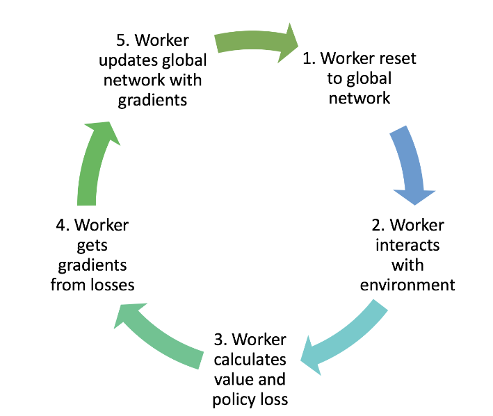
The natural performance optimization to make is what if we didn’t require the workers to wait for others to finish rollouts, allowing the workers to update our global policy asynchronously and providing gradient updates without waiting for all workers each iteration.
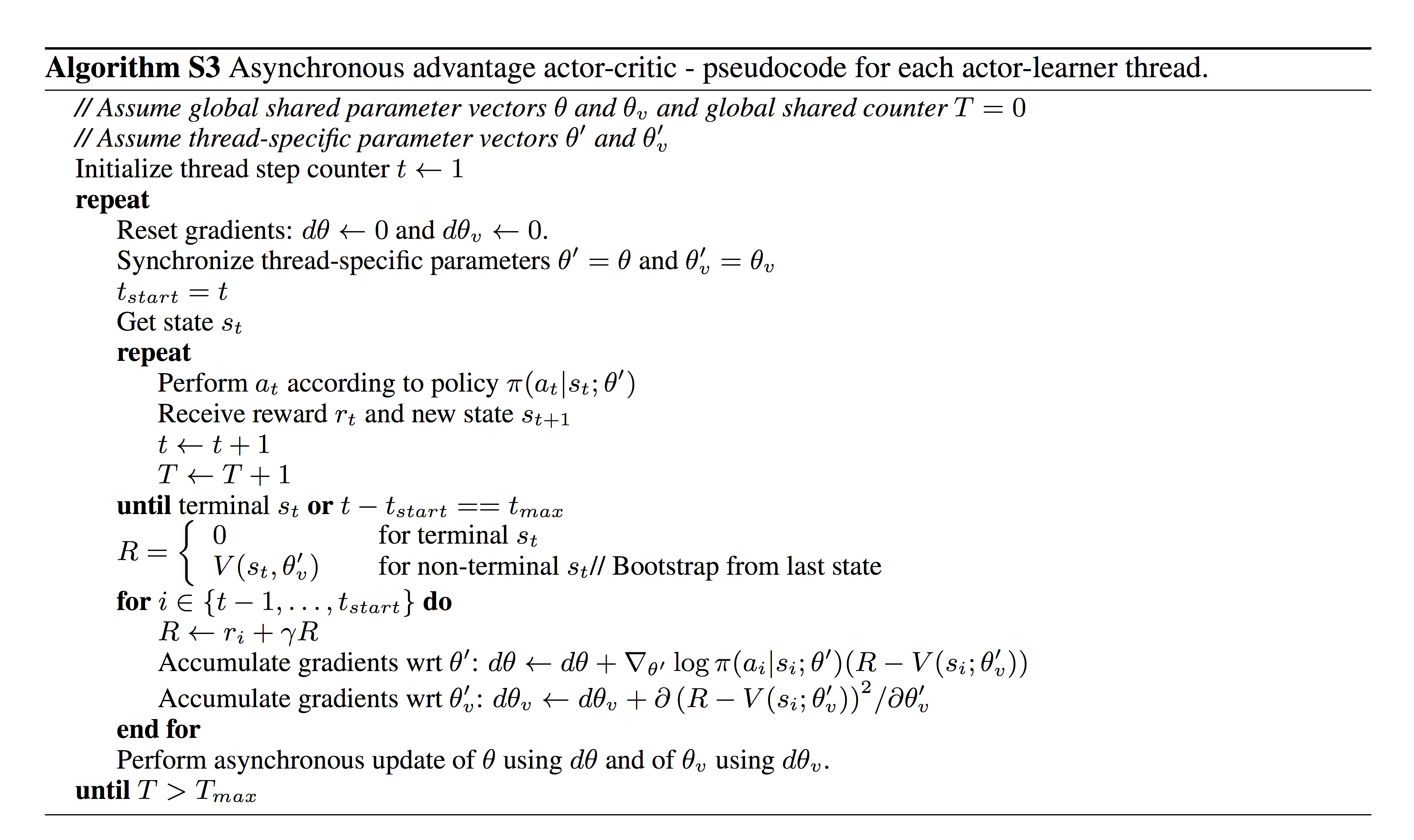
Summarized in algorithmic form, where
\(\theta\) is the global actor parameters and \(\theta_{v}\) is the global critic parameters
\(\theta', \theta'_{v}\) are the thread (worker) specific parameters that may not be in sync with other threads to asynchronous updates
Entropy Regularization
In the A3C paper, entropy regularization is an extra term added to the actor’s objective that rewards stochasticity in the policy. In actor–critic it’s used to prevent the actor from collapsing too early to a near-deterministic (often suboptimal) policy and to improve exploration.
For a discrete action policy \(\pi_{\theta}(\cdot \mid s)\) we have by definition of entropy that
Recall that higher entropy results in more spread-out action probabilities so we want to force a higher entropy term to update our policy objective by adding a regularized entropy term!
PPO is derived from policy improvement logic and more so a approximate policy iteration method than a policy gradient method.
High UTD
let us define the frequency of gradient updates we used in Actor-Critic
\[\text{Updates to Data (UTD)} = \frac{\text{number of gradient updates}}{\text{number of env. steps (samples)}}\]
Obviously it seems to us that a high UTD is efficient with collected data - and a bottleneck in RL for complex environments is exactly data collection - so we want to come up with methods that work well with high UTD. So let’s modify actor-critic to have \(UTD > 1\). But…
if we apply one gradient update step, then we land on a new policy \(\pi'\) parameterized by \(\theta'\). We cannot compute the same policy gradient estimate for \(\nabla_{\theta}U(\theta)\) by reusing the past rollouts (when computing the advantages).
This means that if we forcefully use a high UTD, then we have a noisy estimate based on limited experience and can result in policy drifts. This is a motivator for PPO and TRPO methods as we discuss: What if we constrained our update steps so that the new policy \(\pi'\) is close enough to \(\pi\) and we can reuse the same gradient updates for old set of advantages collected!
Policy Improvement
Performance of Policy
If we quantify the performance of a policy as expected return over all trajectories
and define a discounted state visitation distribution that as the weighted time spent in a specific state \(s\) over all trajectories given a policy \(\pi\)
\(\Pr_{\pi}\) specifically refers to probability over policy (all policy-induced randomness)
the sum of all pmfs for \(d^\pi(s)\) over all states is \(\sum_{s} d^\pi(s) = \frac{1}{1-\gamma}\), because summing over \(s\) sums the inner probability to \(1\) for each time step
The state visitation distribution is important because we can rewrite a discounted sum over time of some some state-dependent function\(f(s)\) as an expectation over the states from the state visitation distribution.
This is a nice identity we can use to reparameterize the trajectory distribution for our performance difference lemma.
Performance Difference Lemma
Then we can show that the policy improvement from \(\pi \rightarrow \pi'\) can be written as expected advantage over state visitation distribution and action sampling from our policy.
If we compute expectation of advantage over all trajectories, we need to expand the expression and reproduce an expression for the global policy difference we are seeking.
To start, for a fixed state \(s\), our advantage expectation over our action distribution from \(\pi'\) is
If we consider this same advantage expectation over \((s_{t}, a_{t})\) generated by \(\pi'\) from \(s_{0} \sim \rho\), then summing this over entire trajectory, we eventually can isolate the performance of both \(\pi\) and \(\pi'\) as performance difference as wanted!
The whole motivation behind PPO is about making safe, stable policy updates while aiming using data collected from ourolder policy\(\pi\). But the issue is our performance difference directly samples directly from \(\pi'\). Can we avoid this?
Importance Sampling
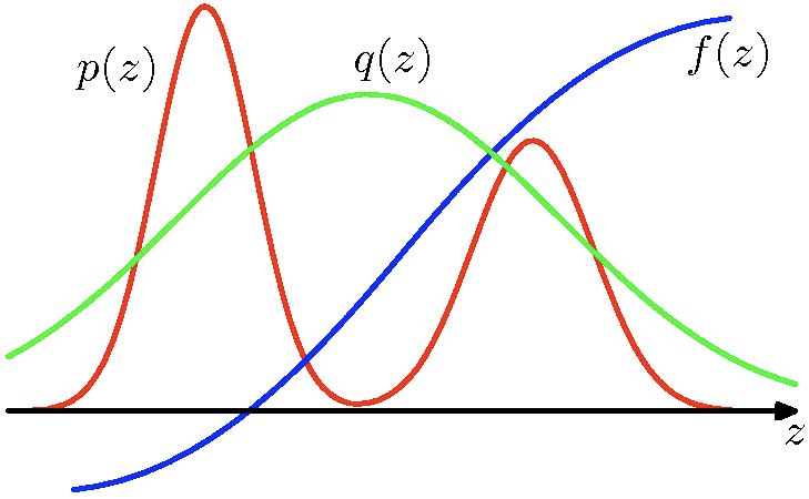
If we can’t sample from \(\pi'\) of a distribution \(p(z)\), but want to compute an expectation of a function \(f(z)\) under that distribution, then a technique called importance sampling allows us to sample from a different easier proposal/behavior distribution \(q(z)\) then scale using a term called important weight on our function values! :
which works as long as the denominator \(q(z) > 0\) whenever \(p(z) > 0\)
And as always we can compute an unbiased estimator for the expectation using Monte Carlo Estimation
Policy Improvement Reformulation
Then to apply this trick to our formulation, we aim to express our expectation entirely in terms of \(\pi\), our first attempt in re-expressing our state visitation distribution in terms of \(\pi\) would be
\[\max_{\pi'} \mathbb{E}_{s \sim d^{\pi'}(s),\ a \sim \pi'(\cdot\mid s)}[A^\pi(s,a)] = \max_{\pi'} \mathbb{E}_{\color{red} s \sim d^\pi(s), a\sim \pi'(\cdot\mid s)}\left[ \frac{d^{\pi'}(s)}{d^\pi(s)}A^\pi (s,a) \right]\]
but calculating state-visitation ratio \(\frac{d^{\pi'}(s)}{d^\pi(s)}\) is hard in itself - because the discounted visitation distribution for \(\pi'\) is unknown - and if we try to estimate this ratio we need a large amount of sampling, and because this is a high variance term that could explode in certain states, this would lead to instability in the computation.
PPO fixes this by simply keeping \(\pi\) close to \(\pi'\) so that the state-visitation distribution naturally induces an approximate equality of \(d^{\pi'}\approx d^\pi\). And we still apply the importance sampling trick for \(\pi'(\cdot\mid s_{t})\) which note the ratio \(\frac{\pi'(\cdot\mid s_{t})}{\pi(\cdot\mid s_{t})}\) is easy to deal with - this is just directly from our policy network!
\[\begin{align*}
\max_{\pi'}\mathbb{E}_{s \sim d^{\pi'}(s), a \sim \pi'(\cdot \mid s_{t})}[A^\pi (s, a)] &= \max_{\pi'} \mathbb{E}_{ \color{red} s \sim d^\pi(s), a \sim \pi'(\cdot \mid s_{t})}\left[ \cancelto{ 1 }{ \frac{d^{\pi'}(s)}{d^\pi(s)} \ }A^\pi(s, a) \right] \tag{PPO assumption} \\
&= \max_{\pi'}\mathbb{E}_{s \sim d^\pi(s), \color{red} a \sim \pi(\cdot \mid s_{t})}\left[ \frac{\pi(a \mid s_{t})}{\pi'(a \mid s_{t})} A^\pi (s, a) \right]
\end{align*}\]
Constrained Maximization Updates
We need to take gradient ascent steps to find the best \(\pi'\), but wait…
We want to reuse the same policy \(\pi\) advantages for multiple policy gradient updates to our parameters \(\theta'\), not just one. But if we blindly follow this gradient, what if we make too big of policy updates to \(\pi'\)? Then actions that were likely under \(\pi\) may not be likely anymore and
the advantages we computed are stale for later updates and
our assumption \(d^{\pi'} \not \approx d^\pi\) may not hold.
PPO aims to enforce some closeness penalty constraints on how far the new policy \(\pi'\) can drift from \(\pi\) on each gradient update! This way we can have high UTD. This can done through adding a regularization term to our objective.
Clipped Ratio Objectives for Constrained Step Size
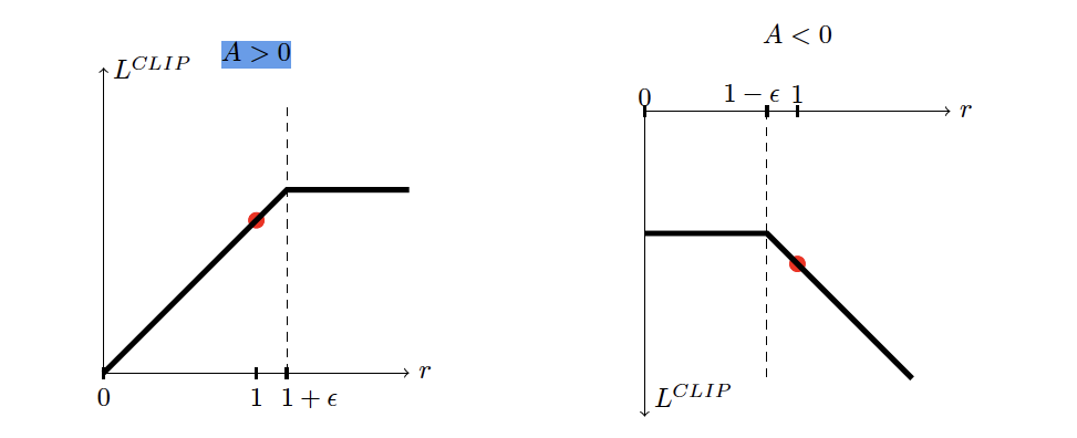
But what PPO actually does is use a soft approximation by utilizing ratio clipping keeping \(\frac{\pi'(a\mid s)}{\pi(a \mid s)}\) close to 1 instead of using an explicit distance metric (KL Divergence) as in TRPO. Remember the whole purpose is to make sure the old batch of trajectories representative of the new policy so we can get high UTD.
But just including a naive clip objectives clips our has the issue of clipping too much, even in useful situations
if our advantage \(A(s_{t},a_{t}) > 0\), even if our ratio \(r < 1 - \epsilon\), \(a_{t}\) is still better than our current baseline in \(\pi\) and the right update is increase its probability
but because the clipped ratio becomes level when \(<1-\epsilon\) , then the gradient zeros out, and we don’t get to use this \((s,a)\) experience for gradient update even though a positive advantage is clearly beneficial for forcing \(\pi'(a \mid s)\) to be higher probability.
If our advantage \(A(s_{t},a_{t}) < 0\), even if our ratio \(r > 1 + \epsilon\) , \(a_{t}\) is still worse than our current baseline and the right update is to decrease its probability
but the naive clipped objective zeros out the gradient once again, and we miss utilizing this \((s,a)\) experience for gradient update, even though a negative advantage is clearly necessary to force \(\pi'(a\mid s)\) smaller.
So our entire clipped objective adds an additional \(\min\) term so that we only clip the ratio only in situations we actually have the issue of over-improving our policy! Now positive advantages with ratio \(r < 1 -\epsilon\) can still be made more probable and negative advantages with ratio \(r > 1+\epsilon\) can still be made less probable.
In summary, this full clipped objective visualized:
If our advantage is positive, then we keep gradient updates up to \(1+\epsilon\)
If our advantage is negative, then we keep gradient updates after \(1- \epsilon\)
Asymmetric clipping
In reality we need to emphasize good actions when exploring for language models, meaning our clip term should be something like
This means that we want to make \(\epsilon_{+} < \epsilon_{-}\) so that we don’t clip for higher positive advantages that we would clip if we kept \(\epsilon_{-}\) fixed and had \(\epsilon_{+} = \epsilon_{-}\)!
GAE - Generalized Advantage Estimation
While we have seen \(n\)-step bootstrapping for computing advantage estimates \(A_{t}^n = r_{t} + \gamma r_{t+1} + \gamma^2r_{t+2} + \dots + \gamma^n V(s_{t+n}) - V(s_{t})\), the tradeoff is while this estimator is less biased, it is higher variance than our high bias, low variance simple TD-estimate \(A_{t}^1 = r_{t} + \gamma V(s_{t+1} )-V(s)\).
Instead of trying to determine the best \(n\)-step TD target to use, GAE computes exponentially weighted sum of all such \(n\)-step targets, but this can also be simplified to a form - weighted sum of 1-step future TD errors starting at \(t\) - that is easier to compute
The parameter \(\lambda \in [0,1]\) allows us to balance bias-variance in our advantage estimates, with a smaller \(\lambda\) having higher bias and lower variance, but a larger \(\lambda\) having lower bias and higher variance.
\(\lambda = 0\), then only the \(l=0\) term is kept in the summation leaving us with 1-step TD of \(\hat{A}_{t} = \delta_{t}\)
\(\lambda \rightarrow 1\), then we care about future TD errors fully reaching something similar to Monte-Carlo
By easier to compute we mean this has a way to conveniently recursively compute each timestep
Then we can compute any \(\hat{A}_{t}\) by iteratively computing backwards from \(t=T-1\) to \(t=0\).
Performance
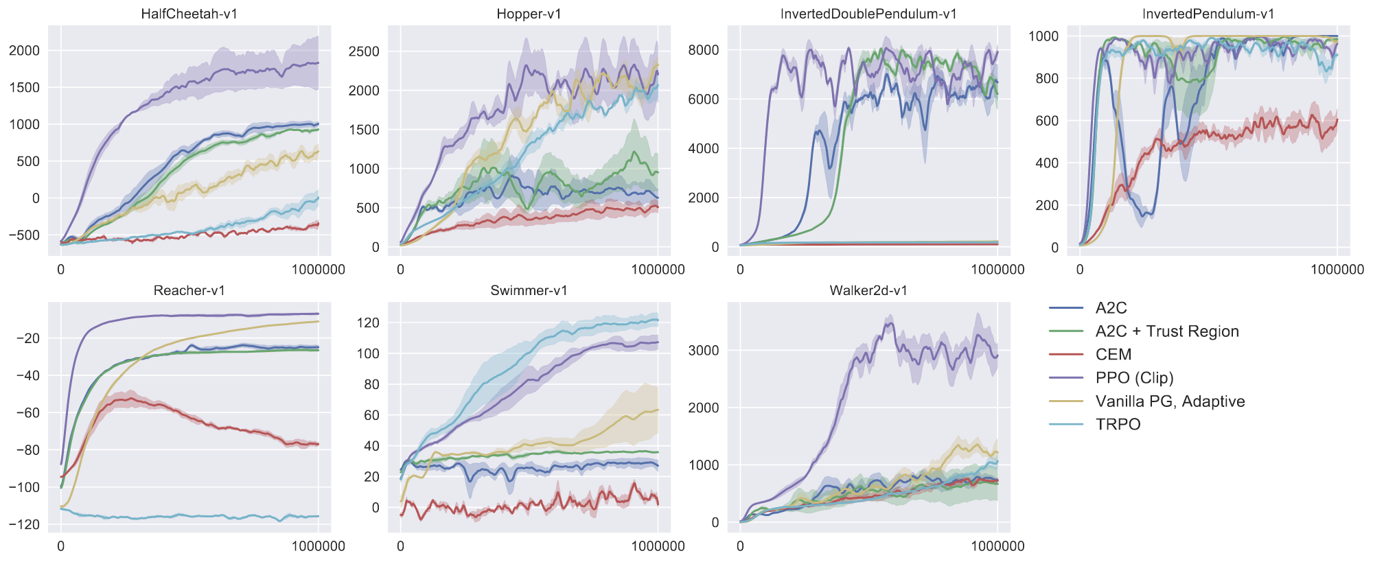
PPO Performance in MuJoCo Tasks
TRPO - Trust-Region Policy Optimization
If we were to keep the KL-constraint in our objective instead of a soft ratio-clipping objective with PPO, then the formulation is different. This is called TRPO.
In optimization problems in general, a trust region is a rule for making small optimization steps to update parameters within a neighborhood where our local approximation is “trusted” to predict improvement.
With KL we have defined our neighborhood in terms of policy space measured through KL divergence.
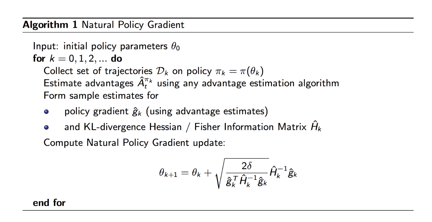
Natural Policy Gradient
We can convert this constrain into a penalty, just adding the KL term, so we can just perform unconstrained approximation. We can then approximate this objective by
estimating the policy objective with a first order Taylor expansion and
estimating the KL term with a second order Taylor expansion
For the second order KL Term, we solve in which the inner term is called the fisher information matrix: the Hessian of the KL divergence at the point where the two distributions match.
We essentially want to find the optimal \(\mathbf{d}\) for our objective which can be done through finding local minimnum
\[\begin{aligned}
% --- Substitute Fisher (2nd-order KL) into the constrained problem via Lagrangian ---
\mathbf d^*
&= \arg\max_{\mathbf d}\;\nabla_\theta U(\theta)\Big|_{\theta=\theta_{\mathrm{old}}}^{\top}\mathbf d
\;-\;\frac{1}{2}\lambda\,\mathbf d^{\top}\mathbf F(\theta_{\mathrm{old}})\mathbf d \\
&= \arg\min_{\mathbf d}\;-\nabla_\theta U(\theta)\Big|_{\theta=\theta_{\mathrm{old}}}^{\top}\mathbf d
\;+\;\frac{1}{2}\lambda\,\mathbf d^{\top}\mathbf F(\theta_{\mathrm{old}})\mathbf d
\\[10pt]
% --- Solve by setting gradient wrt d to zero ---
\mathbf 0
&= \nabla_{\mathbf d}\left(
-\nabla_\theta U(\theta)\Big|_{\theta=\theta_{\mathrm{old}}}^{\top}\mathbf d
+\frac{1}{2}\lambda\,\mathbf d^{\top}\mathbf F(\theta_{\mathrm{old}})\mathbf d
\right) \\
&= -\nabla_\theta U(\theta)\Big|_{\theta=\theta_{\mathrm{old}}}
+\frac{1}{2}\lambda\left(\mathbf F(\theta_{\mathrm{old}})+\mathbf F(\theta_{\mathrm{old}})^{\top}\right)\mathbf d \\
&= -\nabla_\theta U(\theta)\Big|_{\theta=\theta_{\mathrm{old}}}
+\lambda\,\mathbf F(\theta_{\mathrm{old}})\mathbf d
\qquad (\mathbf F \text{ symmetric})
\\[8pt]
\Rightarrow\quad
\mathbf d
&= \frac{1}{\lambda}\,\mathbf F(\theta_{\mathrm{old}})^{-1}\nabla_\theta U(\theta)\Big|_{\theta=\theta_{\mathrm{old}}}
\\[10pt]
% --- Natural gradient direction and parameter update ---
\mathbf g_N
&:= \mathbf F(\theta_{\mathrm{old}})^{-1}\nabla_\theta U(\theta)\Big|_{\theta=\theta_{\mathrm{old}}} \\
\theta_{\mathrm{new}}
&= \theta_{\mathrm{old}} + \alpha\,\mathbf g_N
\end{aligned}\]
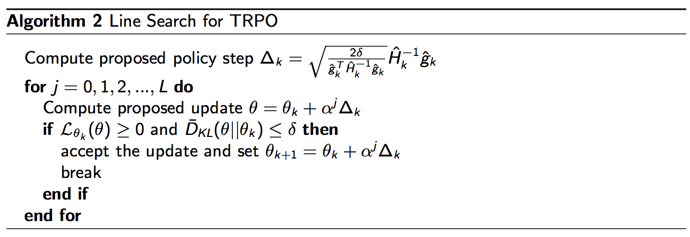
How shall we choose the step size along the natural gradient direction? From the 2nd order Taylor expansion of the KL term, given that we require our KL between new and old policies to be at most \(\epsilon\), then we can directly solve for \(\alpha\)
Because the quadratic KL approximation is in the end just an approximation that is done with neural nets, the actual KL may not actually be \(\leq \epsilon\) like we want it. Instead we try something that just tests different step sizes \(\alpha^{j+1} = c\,\alpha^j\) with a shrink factor \(c \in (0,1)\) to gauge a KL constraint that works and a positive surrogate improvement.