Overview

Actor-Critic methods build off even further from our state-dependent baselines used in REINFORCE with baselines method where our action advantage is \(A^\pi (s_{t}^i, a_{t}^i) = G_{t}^{(i)} - V_{\phi}^\pi(s_{t}^i)\)

But the \(G_{t}^{(i)}\) term can still have high variance: it’s a single rollout Monte-Carlo return based on our \(s_{t}\) and \(a_{t}\) and varies for different trials in our environment; but doesn’t this term sound familiar?

Our returns \(G_{t} = \sum_{k=t}^T R(s_{k}, a_{k})\) are exactly estimated by our Q-functions \(Q^\pi(s,a) = \mathbb{E}[G_{t} \mid s_{t}, a_{t}]\) by definition!

Moreover, since our baseline is our value functions \(V_{\phi}^\pi(s)\), then we should expand our bellman equations to express Q-functions in terms of value functions: \(Q^\pi(s,a) = \mathbb{E}[G_{t} \mid s_{t}, a_{t}] = \mathbb{E}[R_{t} + \gamma G_{t+1} \mid s_{t}, a_{t}] = \mathbb{E}[R_{t}+\gamma V(s_{t+1}) \mid s_{t},a_{t}]\). This way we avoid having to update two critic networks - and only need one critic network that estimates \(V_{\phi}^\pi(s)\)!

Then our action advantages can be simplified through TD-bootstrapping as

\[A^\pi(s_{t}^i, a_{t}^i) = Q(s_{t},a_{t}) - V_{\phi}^\pi(s_{t}) = R(s_{t}^i, a_{t}^i)+ \gamma V_{\phi}^\pi(s_{t+1}^{i}) - V_{\phi}^\pi(s_{t})\]

This critic “critiques” the actor’s choices by providing an baseline evaluation signal - advantage - that guides how the actor should change.

Initialize actor policy parameters \(\theta\) and critic parameters \(\phi\)
Sample trajectories \(\{\tau_{i} = \{s_{t}^i , a_{t}^i\}_{i=0}^T \}\) by deploying our current policy \(\pi_{\theta}(a_{t} \mid s_{t})\)
Compute returns \(G_t^{(i)} = \sum_{k=t}^{T-1}\gamma^{k-t} r(s_k^{(i)},a_k^{(i)})\) for all \(i,t\)
Fit critic value functions \(V_{\phi}^\pi(s)\) through MC or TD estimation to update the critic \(\phi\)
Compute action advantage estimates: \(A^\pi (s_{t}^i, a_{t}^i) = G_{t}^{(i)} - V_{\phi}^\pi(s_{t}^i)\) for all \(i,t\)
\(\nabla_\theta U(\theta)\approx \frac{1}{N}\sum_{i=1}^N\sum_{t=0}^{T-1}\nabla_\theta \log \pi_\theta(a_t^{(i)}\mid s_t^{(i)})\,\hat A_t^{(i)}\)
\(\theta \leftarrow \theta + \alpha \nabla_{\theta}U(\theta)\)

In some sense the actor-critic is just “policy iteration” written in gradient form.

We run the policy and collect a series of \(N\) trajectories.
Based on the performance, we compute advantages for each time step during each trajectory and take note of high advantage \(A^\pi\) actions - where \(Q_{\pi}(s,a)\) value is higher than the state \(V_{\pi}(s)\) value.
Then we update our policy parameters \(\pi \rightarrow \pi_{new}\) directly using a policy gradient that is computed through these advantages so that the policy makes those high advantage actions more probable.

A2C - Advantage Actor-Critic (Distributed Synchronous)

The trajectories we collect arrive sequentially, and successive on-policy updates can be highly correlated because they come from a single evolving policy interacting with the environment. We have seen how in off-policy methods like DQN, replay buffers help decorrelate data, so for on-policy actor-critic methods, we instead collect experience in parallel.

In A2C, we parallelize experience collection across multiple workers and aggregate their rollouts into a single batch before computing one single global gradient update, and synchronizing the updated policy globally to all workers. Because each workers interacts with the environment differently, then aggregating their updates removes the problem of correlation, while simultaneously reducing data collection time!

So, each worker runs the current policy to generate trajectories and compute gradient contributions from its own rollouts. We then synchronize: the global update is applied only after all workers finish and their gradients are combined, yielding more diverse experience per update and more stable training!

This distributed synchronous, because all workers collect trajectories only after synchronizing a global policy to use.

A3C - Asynchronous Advantage Actor-Critic (Distributed Asynchronous)

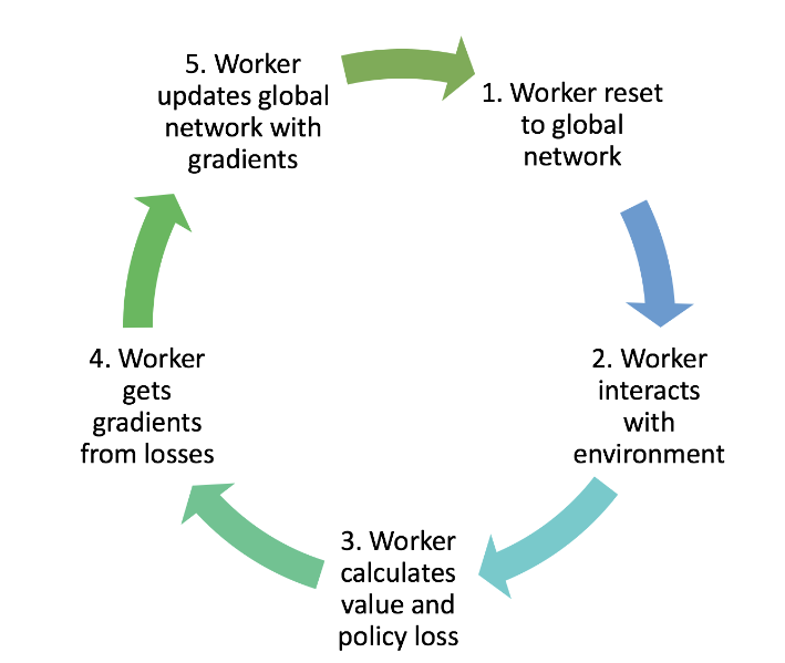
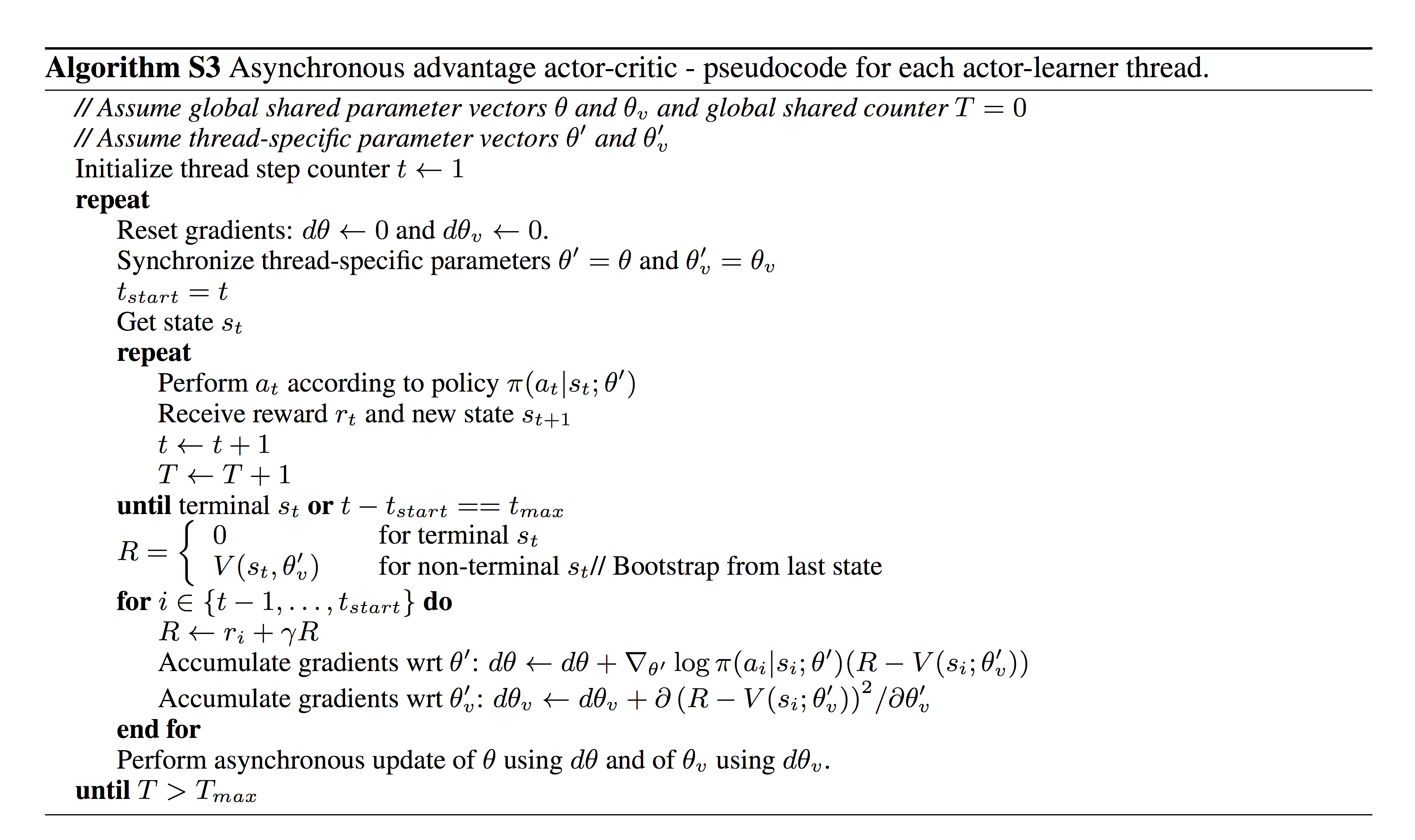
The natural performance optimization to make is what if we didn’t require the workers to wait for others to finish rollouts, allowing the workers to update our global policy asynchronously and providing gradient updates without waiting for all workers each iteration.

Summarized in algorithmic form, where

\(\theta\) is the global actor parameters and \(\theta_{v}\) is the global critic parameters
\(\theta', \theta'_{v}\) are the thread (worker) specific parameters that may not be in sync with other threads to asynchronous updates

Entropy Regularization

In the A3C paper, entropy regularization is an extra term added to the actor’s objective that rewards stochasticity in the policy. In actor–critic it’s used to prevent the actor from collapsing too early to a near-deterministic (often suboptimal) policy and to improve exploration.

For a discrete action policy \(\pi_{\theta}(\cdot \mid s)\) we have by definition of entropy that

\[H(\pi_\theta(\cdot\mid s)) \;=\; -\sum_a \pi_\theta(a\mid s)\,\log \pi_\theta(a \mid s)\]

Recall that higher entropy results in more spread-out action probabilities so we want to force a higher entropy term to update our policy objective by adding a regularized entropy term!

\[U_{\text{ent}}(\theta)=\mathbb{E}\Big[\sum_t \big(\log \pi_\theta(a_t\mid s_t)\,\hat A_t + \beta\,H(\pi_\theta(\cdot\mid s_t))\big)\Big].\]

For our gradient updates then:

\[\begin{flalign} \nabla_{\theta}\, H \!\left(\pi_{\theta}(\cdot \mid s)\right) &= - \sum_{a}\Big[\,\nabla_{\theta}\pi_{\theta}(a\mid s)\big(\log \pi_{\theta}(a\mid s)+1\big)\Big] \tag{product rule for derivatives} \\ &= - \mathbb{E}_{a\sim \pi_{\theta}(\cdot\mid s)} \Big[\,\nabla_{\theta}\log \pi_{\theta}(a\mid s)\,\big(\log \pi_{\theta}(a\mid s)+1\big)\Big] \end{flalign}\]

And substituting we get!

\[\begin{aligned} \nabla_{\theta} U_{ent}(\theta) = \mathbb{E}\Bigg[ \sum_{t}\nabla_{\theta}\log \pi_{\theta}(a_t\mid s_t)\,\hat{A}_t - \beta\,\mathbb{E}_{a\sim \pi_{\theta}(\cdot\mid s_t)} \Big[\nabla_{\theta}\log \pi_{\theta}(a\mid s_t)\big(\log \pi_{\theta}(a\mid s_t)+1\big)\Big] \Bigg]. \end{aligned}\]

PPO - Proximal Policy Optimization

PPO is derived from policy improvement logic and more so a approximate policy iteration method than a policy gradient method.

High UTD

let us define the frequency of gradient updates we used in Actor-Critic

\[\text{Updates to Data (UTD)} = \frac{\text{number of gradient updates}}{\text{number of env. steps (samples)}}\]

Obviously it seems to us that a high UTD is efficient with collected data - and a bottleneck in RL for complex environments is exactly data collection - so we want to come up with methods that work well with high UTD. So let’s modify actor-critic to have \(UTD > 1\). But…

Here’s the issue:

\[\theta \leftarrow \theta + \alpha \nabla_{\theta}U(\theta)\]

if we apply one gradient update step, then we land on a new policy \(\pi'\) parameterized by \(\theta'\). We cannot compute the same policy gradient estimate for \(\nabla_{\theta}U(\theta)\) by reusing the past rollouts (when computing the advantages).

This means that if we forcefully use a high UTD, then we have a noisy estimate based on limited experience and can result in policy drifts. This is a motivator for PPO and TRPO methods as we discuss: What if we constrained our update steps so that the new policy \(\pi'\) is close enough to \(\pi\) and we can reuse the same gradient updates for old set of advantages collected!

Policy Improvement

Performance of Policy

If we quantify the performance of a policy as expected return over all trajectories

\[J(\pi) = \mathbb{E}\left[ \sum_{t=0}^\infty \gamma^t r(s_{t}, a_{t}) \right] = \mathbb{E}_{s_{0} \sim \rho}[V^\pi(s_{0})]\]

and define a discounted state visitation distribution that as the weighted time spent in a specific state \(s\) over all trajectories given a policy \(\pi\)

\[d^\pi(s) = \sum_{t=0}^\infty \gamma^t \Pr_{\pi} (s_{t} = s \mid s_{0} \sim \rho)\]

where

\(\Pr_{\pi}\) specifically refers to probability over policy (all policy-induced randomness)
the sum of all pmfs for \(d^\pi(s)\) over all states is \(\sum_{s} d^\pi(s) = \frac{1}{1-\gamma}\), because summing over \(s\) sums the inner probability to \(1\) for each time step

The state visitation distribution is important because we can rewrite a discounted sum over time of some some state-dependent function \(f(s)\) as an expectation over the states from the state visitation distribution.

\[\sum_{t=0}^\infty \gamma^t \mathbb{E}_\pi[f(S_t)] = \sum_{t=0}^\infty \gamma^t \sum_s f(s)\Pr_\pi(S_t=s) = \sum_s f(s)\underbrace{\sum_{t=0}^\infty \gamma^t \Pr_\pi(S_t=s)}_{d^{\pi}(s)} = \mathbb{E}_{s \sim d_{\pi}(s)} [f(s)]\]

This is a nice identity we can use to reparameterize the trajectory distribution for our performance difference lemma.

Performance Difference Lemma

Then we can show that the policy improvement from \(\pi \rightarrow \pi'\) can be written as expected advantage over state visitation distribution and action sampling from our policy.

\[J(\pi') - J(\pi) = \mathbb{E}_{\tau\sim\pi'}\left[\sum_{t=0}^\infty \gamma^t A^\pi(s_t,a_t)\right] = \mathbb{E}_{s \sim d^{\pi'},\ a \sim \pi'(\cdot \mid s)}[A^\pi (s,a)]\]

Intuitively this is true because the advantage \(A^\pi(s,a) = Q^\pi(s,a) - V^\pi(s)\) is a single-step improvement signal:

It measures the difference

take \(a\) - sampled from \(\pi'\) - at \(s\) then follow \(\pi\)
follow \(\pi\) immediately from \(s\) And we are averaging this over the entire joint \((s,a)\) distribution of our new policy \(\pi'\)

Proof

Let’s start from the definition of advantage expanded using Bellman

\[A^\pi(s,a) = Q^\pi(s,a) - V^\pi(s) = r(s,a) + \gamma \mathbb{E}_{s' \sim P(\cdot \mid s,a)}[V^\pi(s')] - V^\pi(s)\]

If we compute expectation of advantage over all trajectories, we need to expand the expression and reproduce an expression for the global policy difference we are seeking.

To start, for a fixed state \(s\), our advantage expectation over our action distribution from \(\pi'\) is

\[\mathbb{E}_{a \sim \pi'}[A^\pi(s,a)] = \mathbb{E}_{a \sim \pi'}[r(s,a)] + \gamma \mathbb{E}_{a \sim \pi',\ s' \sim P(\cdot \mid s ,a )}[V^\pi(s')] - \mathbb{E}_{a \sim \pi'}[V^\pi(s)] \\\]

If we consider this same advantage expectation over \((s_{t}, a_{t})\) generated by \(\pi'\) from \(s_{0} \sim \rho\), then summing this over entire trajectory, we eventually can isolate the performance of both \(\pi\) and \(\pi'\) as performance difference as wanted!

\[\begin{flalign} & \sum_{t=0}^\infty \gamma^t \mathbb{E}_{\pi'}[A^\pi(s_{t},a_{t})] = \sum_{t=0}^\infty \gamma^t \mathbb{E_{\pi'}}[r(s_{t},a_{t})] + \underbrace{ \sum_{t=0}^\infty \gamma^{t+1} \mathbb{E}_{\pi'}[V^\pi(s_{t+1})] - \sum_{t=0}^\infty \gamma^t \mathbb{E}_{\pi'}[V^\pi(s_{t})] }_{ \sum_{t=1}^\infty \gamma^{t} \mathbb{E}_{\pi'}[V^\pi(s_{t})] - \sum_{t=0}^\infty \gamma^t \mathbb{E}_{\pi'}[V^\pi(s_{t})] = \boxed{-\mathbb{E}_{\pi'}[V^\pi(s_{0})]} } \tag{telescoping!} \\ & \mathbb{E}_{s \sim d^{\pi'}(s),\ a\sim \pi'(\cdot \mid s)}[A^\pi(s_{t},a_{t})] = \mathbb{E}_{s \sim d^{\pi'}(s), a \sim \pi'(\cdot \mid s)}[r(s_{t},a_{t})] - \underbrace{ \mathbb{E}_{s_{0} \sim \rho(s_{0})}[V^\pi(s_{0})] }_{ s_{0} \text{ doesn't depend on policy} } \tag{convert discounted sums!} \\ & \mathbb{E}_{s \sim d^{\pi'}(s),\ a\sim \pi'(\cdot \mid s)}[A^\pi(s_{t},a_{t})] = J(\pi') - J(\pi) \tag{substitute} \end{flalign}\]

Policy Improvement Formulation

We aim to find a new policy \(\pi'\) maximizing our policy improvement:

\[\max_{\pi'}J(\pi') = \max_{\pi'}(J(\pi') - J(\pi)) = \max_{\pi'} \mathbb{E}_{s \sim d'^\pi(s), a \sim \pi'(\cdot \mid s)}[A^\pi(s, a)]\]

The whole motivation behind PPO is about making safe, stable policy updates while aiming using data collected from our older policy \(\pi\). But the issue is our performance difference directly samples directly from \(\pi'\). Can we avoid this?

Importance Sampling

If we can’t sample from \(\pi'\) of a distribution \(p(z)\), but want to compute an expectation of a function \(f(z)\) under that distribution, then a technique called importance sampling allows us to sample from a different easier proposal/behavior distribution \(q(z)\) then scale using a term called important weight on our function values! :

\[\begin{align*} \mathbb{E}_{z \sim p(z)}[f(z)] = \int f(z) p(z) dz = \int q(z) f(z) \underbrace{ \frac{p(z)}{q(z)} }_{ \text{weight} } dz = \mathbb{E}_{z \sim q(z)}\left[ f(z) \frac{p(z)}{q(z)} \right] \end{align*}\]

which works as long as the denominator \(q(z) > 0\) whenever \(p(z) > 0\)

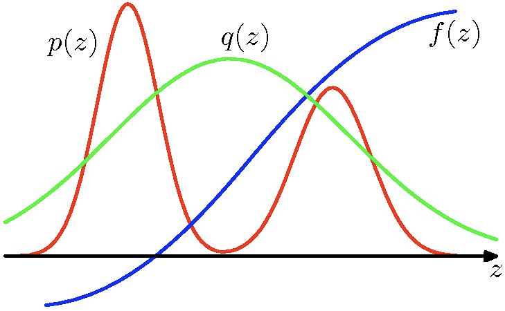
And as always we can compute an unbiased estimator for the expectation using Monte Carlo Estimation

Policy Improvement Reformulation

Then to apply this trick to our formulation, we aim to express our expectation entirely in terms of \(\pi\), our first attempt in re-expressing our state visitation distribution in terms of \(\pi\) would be

\[\max_{\pi'} \mathbb{E}_{s \sim d^{\pi'}(s),\ a \sim \pi'(\cdot\mid s)}[A^\pi(s,a)] = \max_{\pi'} \mathbb{E}_{\color{red} s \sim d^\pi(s), a\sim \pi'(\cdot\mid s)}\left[ \frac{d^{\pi'}(s)}{d^\pi(s)}A^\pi (s,a) \right]\]

but calculating state-visitation ratio \(\frac{d^{\pi'}(s)}{d^\pi(s)}\) is hard in itself - because the discounted visitation distribution for \(\pi'\) is unknown - and if we try to estimate this ratio we need a large amount of sampling, and because this is a high variance term that could explode in certain states, this would lead to instability in the computation.

PPO fixes this by simply keeping \(\pi\) close to \(\pi'\) so that the state-visitation distribution naturally induces an approximate equality of \(d^{\pi'}\approx d^\pi\). And we still apply the importance sampling trick for \(\pi'(\cdot\mid s_{t})\) which note the ratio \(\frac{\pi'(\cdot\mid s_{t})}{\pi(\cdot\mid s_{t})}\) is easy to deal with - this is just directly from our policy network!

\[\begin{align*} \max_{\pi'}\mathbb{E}_{s \sim d^{\pi'}(s), a \sim \pi'(\cdot \mid s_{t})}[A^\pi (s, a)] &= \max_{\pi'} \mathbb{E}_{ \color{red} s \sim d^\pi(s), a \sim \pi'(\cdot \mid s_{t})}\left[ \cancelto{ 1 }{ \frac{d^{\pi'}(s)}{d^\pi(s)} \ }A^\pi(s, a) \right] \tag{PPO assumption} \\ &= \max_{\pi'}\mathbb{E}_{s \sim d^\pi(s), \color{red} a \sim \pi(\cdot \mid s_{t})}\left[ \frac{\pi(a \mid s_{t})}{\pi'(a \mid s_{t})} A^\pi (s, a) \right] \end{align*}\]

Constrained Maximization Updates

We need to take gradient ascent steps to find the best \(\pi'\), but wait…

\[\begin{align*} & \max_{\pi'} \mathbb{E}_{s \sim d^\pi,\ a \sim \pi(\cdot \mid s)} \left[\frac{\pi_{\theta'}(a \mid s)}{\pi(a \mid s)}\,A^\pi(s,a)\right] \\ & \nabla_{\theta'} \mathbb{E}_{s \sim d^\pi,\ a \sim \pi(\cdot \mid s)} \left[\nabla_{\theta'}\left(\frac{\pi_{\theta'}(a \mid s)}{\pi(a \mid s)}\right) A^\pi(s,a)\right] \\ &= \mathbb{E}_{s \sim d^\pi,\ a \sim \pi(\cdot \mid s)} \left[\frac{\pi_{\theta'}(a \mid s)}{\pi(a \mid s)}\,\nabla_{\theta'} \log \pi_{\theta'}(a \mid s)\,A^\pi(s,a)\right]. \end{align*}\]

We want to reuse the same policy \(\pi\) advantages for multiple policy gradient updates to our parameters \(\theta'\), not just one. But if we blindly follow this gradient, what if we make too big of policy updates to \(\pi'\)? Then actions that were likely under \(\pi\) may not be likely anymore and

the advantages we computed are stale for later updates and
our assumption \(d^{\pi'} \not \approx d^\pi\) may not hold.

PPO aims to enforce some closeness penalty constraints on how far the new policy \(\pi'\) can drift from \(\pi\) on each gradient update! This way we can have high UTD. This can done through adding a regularization term to our objective.

\[\mathbb{E}_{s \sim d^\pi(s)}\mathbb{E}_{a \sim \pi(\cdot \mid s)}\left[ \frac{ \nabla_{\theta'} \log\pi'(a \mid s)}{\pi(a \mid s)} A^\pi(s,a) \right] - \color{red} \lambda \mathbb{E}_{s}[D(\pi(\cdot \mid s), \pi'(\cdot\mid s))]\]

Clipped Ratio Objectives for Constrained Step Size

But what PPO actually does is use a soft approximation by utilizing ratio clipping keeping \(\frac{\pi'(a\mid s)}{\pi(a \mid s)}\) close to 1 instead of using an explicit distance metric (KL Divergence) as in TRPO. Remember the whole purpose is to make sure the old batch of trajectories representative of the new policy so we can get high UTD.

This clipped objective can be summarized as

\[\max_{\pi'} \mathbb{E}_{s \sim d^\pi(s)} \mathbb{E}_{a \sim \pi(\cdot \mid s)} \left[ \min\left( \frac{\pi'(a\mid s)}{\pi(a\mid s)} A^\pi(s,a) , clip\left( \frac{\pi'(a \mid s)}{\pi(a\mid s)}, 1-\epsilon , 1+\epsilon\right) A^\pi(s,a) \right) \right]\]

A lot is going on here. The intuition is to clip the importance weight \(\frac{\pi'(a\mid s)}{\pi(a \mid s)} \in [1-\epsilon, 1+ \epsilon]\)

\[\operatorname{clip}(f(x),a,b)= \begin{cases} a & f(x)\le a\\ f(x) & a <f(x) <b\\ b & f(x)\ge b \end{cases}\]

Clip directly prevents any gradient updates from occurring outside the intended range \([a,b]\).

\[\frac{d}{dx}\operatorname{clip}(f(x),a,b)= \begin{cases} 0 & f(x)\le a\\ f'(x) & a< f(x) <b\\ 0 & f(x)\ge b \end{cases}\]

But just including a naive clip objectives clips our has the issue of clipping too much, even in useful situations

if our advantage \(A(s_{t},a_{t}) > 0\), even if our ratio \(r < 1 - \epsilon\), \(a_{t}\) is still better than our current baseline in \(\pi\) and the right update is increase its probability but because the clipped ratio becomes level when \(<1-\epsilon\) , then the gradient zeros out, and we don’t get to use this \((s,a)\) experience for gradient update even though a positive advantage is clearly beneficial for forcing \(\pi'(a \mid s)\) to be higher probability.
If our advantage \(A(s_{t},a_{t}) < 0\), even if our ratio \(r > 1 + \epsilon\) , \(a_{t}\) is still worse than our current baseline and the right update is to decrease its probability but the naive clipped objective zeros out the gradient once again, and we miss utilizing this \((s,a)\) experience for gradient update, even though a negative advantage is clearly necessary to force \(\pi'(a\mid s)\) smaller.

So our entire clipped objective adds an additional \(\min\) term so that we only clip the ratio only in situations we actually have the issue of over-improving our policy! Now positive advantages with ratio \(r < 1 -\epsilon\) can still be made more probable and negative advantages with ratio \(r > 1+\epsilon\) can still be made less probable.

In summary, this full clipped objective visualized:

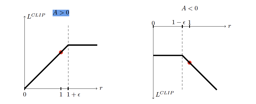
If our advantage is positive, then we keep gradient updates up to \(1+\epsilon\)
If our advantage is negative, then we keep gradient updates after \(1- \epsilon\)

Asymmetric clipping

In reality we need to emphasize good actions when exploring for language models, meaning our clip term should be something like

\[clip\left( \frac{\pi'(s\mid a)}{\pi(s \mid a)}, 1-\epsilon_{-}, 1+ \epsilon_{+} \right)\]

This means that we want to make \(\epsilon_{+} < \epsilon_{-}\) so that we don’t clip for higher positive advantages that we would clip if we kept \(\epsilon_{-}\) fixed and had \(\epsilon_{+} = \epsilon_{-}\)!

GAE - Generalized Advantage Estimation

While we have seen \(n\)-step bootstrapping for computing advantage estimates \(A_{t}^n = r_{t} + \gamma r_{t+1} + \gamma^2r_{t+2} + \dots + \gamma^n V(s_{t+n}) - V(s_{t})\), the tradeoff is while this estimator is less biased, it is higher variance than our high bias, low variance simple TD-estimate \(A_{t}^1 = r_{t} + \gamma V(s_{t+1} )-V(s)\).

\[\begin{array}{c|c|c} n & G_t & \text{Notes} \\ \hline n=1 & G_t^{(1)} = R_{t+1} + \gamma V(S_{t+1}) & \text{TD learning} \\ n=2 & G_t^{(2)} = R_{t+1} + \gamma R_{t+2} + \gamma^{2} V(S_{t+2}) & \\ \vdots & \vdots & \\ n=n & G_t^{(n)} = R_{t+1} + \gamma R_{t+2} + \cdots + \gamma^{n-1} R_{t+n} + \gamma^{n} V(S_{t+n}) & \\ \vdots & \vdots & \\ n=\infty & G_t^{(\infty)} = R_{t+1} + \gamma R_{t+2} + \cdots + \gamma^{T-t-1} R_T + \gamma^{T-t} V(S_T) & \text{MC estimation} \end{array}\]

Instead of trying to determine the best \(n\)-step TD target to use, GAE computes exponentially weighted sum of all such \(n\)-step targets, but this can also be simplified to a form - weighted sum of 1-step future TD errors starting at \(t\) - that is easier to compute

\[\begin{align*} \hat{A}_{t} &= (1-\lambda)\sum_{n=1}^{T-t-1} \lambda^{n-1} G_{t}^{(n)} = \sum_{l=0}^{T-t-1} (\gamma \lambda)^l \delta_{t+l} \\ & \delta_{t} = r_{t} + \gamma V(s_{t+1}) - V(s_{t}) \\ \end{align*}\]

The parameter \(\lambda \in [0,1]\) allows us to balance bias-variance in our advantage estimates, with a smaller \(\lambda\) having higher bias and lower variance, but a larger \(\lambda\) having lower bias and higher variance.

\(\lambda = 0\), then only the \(l=0\) term is kept in the summation leaving us with 1-step TD of \(\hat{A}_{t} = \delta_{t}\)
\(\lambda \rightarrow 1\), then we care about future TD errors fully reaching something similar to Monte-Carlo

By easier to compute we mean this has a way to conveniently recursively compute each timestep

\[\begin{align*} & \hat{A}_{t} = \delta_{t} + \gamma \lambda \sum_{l=0}^{T-(t+1)-1 } (\gamma \lambda)^l \delta_{t+1+l} = \delta_{t} + \gamma \lambda \hat{A}_{t+1} \\ & \hat{A}_{T-1} = \delta_{T-1} \end{align*}\]

Then we can compute any \(\hat{A}_{t}\) by iteratively computing backwards from \(t=T-1\) to \(t=0\).

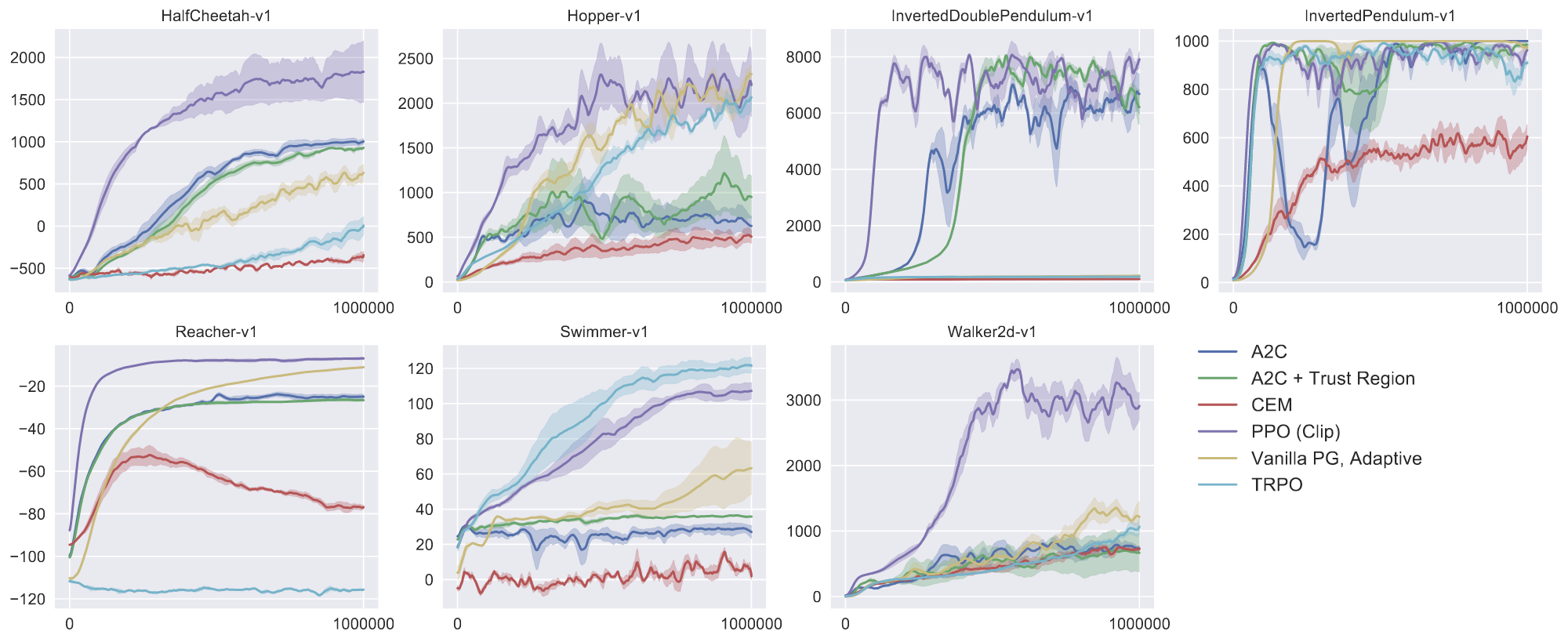
Performance

TRPO - Trust-Region Policy Optimization

If we were to keep the KL-constraint in our objective instead of a soft ratio-clipping objective with PPO, then the formulation is different. This is called TRPO.

Our surrogate objective is now

\[\begin{gather*} \max_{\theta} \mathbb{A}_{\pi_{old}}(\pi) = \sum_{t=1}^T \mathbb{E}_{{s_{t} \sim p_{\theta_{old}}(s_{t})}}\mathbb{E}_{a_{t} \sim \pi_{\theta_{old}}(a_{t} \mid s_{t})}\left[ \frac{\pi_{\theta}(a_{t}\mid s_{t})}{\pi_{\theta_{old}}(a_{t}\mid s_{t})}A^{\pi_{old}}(s_{t}, a_{t}) \right]\\ \text{with regularization constraint } \mathbb{E}_{t}[D_{KL}[\pi_{\theta_{old}}(\cdot\mid s_{t}) \parallel \pi_{\theta}(\cdot \mid s_{t})]] \leq \epsilon \end{gather*}\]

In optimization problems in general, a trust region is a rule for making small optimization steps to update parameters within a neighborhood where our local approximation is “trusted” to predict improvement.

With KL we have defined our neighborhood in terms of policy space measured through KL divergence.

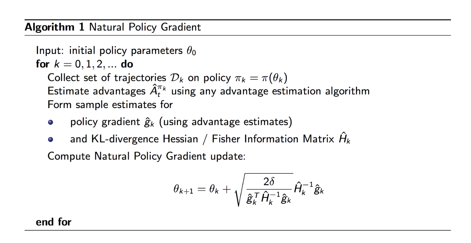
Natural Policy Gradient

We can convert this constrain into a penalty, just adding the KL term, so we can just perform unconstrained approximation. We can then approximate this objective by

estimating the policy objective with a first order Taylor expansion and
estimating the KL term with a second order Taylor expansion

\[\begin{flalign} d^* &= \arg \max_{d} U(\theta + d) - \lambda(D_{KL}[\pi_{\theta} \mid \pi_{\theta+d}] - \epsilon) \\ &\approx \arg \max_{d} U(\theta_{old}) + \nabla_{\theta} U(\theta)\mid_{\theta=\theta_{old}} \cdot d - \frac{1}{2} \lambda (d^T \nabla_{\theta}^2 D_{KL}[\pi_{\theta_{old}} \parallel \pi_{\theta}] + \lambda \epsilon) \end{flalign}\]

Let’s derive the Taylor approximation for the KL term:

\[D_{\mathrm{KL}}(P_{\theta_{\text{old}}} \,\|\, P_\theta) \;\approx\; D_{\mathrm{KL}}(P_{\theta_{\text{old}}} \,\|\, P_{\theta_{\text{old}}}) + \mathbf{d}^\top \nabla_\theta D_{\mathrm{KL}}(P_{\theta_{\text{old}}} \,\|\, P_\theta)\Big|_{\theta=\theta_{\text{old}}} + \frac{1}{2} \mathbf{d}^\top \nabla_\theta^2 D_{\mathrm{KL}}(P_{\theta_{\text{old}}} \,\|\, P_\theta)\Big|_{\theta=\theta_{\text{old}}} \mathbf{d}\]

For the first order KL term:

\[\begin{aligned} % --- gradient term is zero at \theta_{\text{old}} --- \nabla_{\theta}D_{\mathrm{KL}}\!\left(P_{\theta_{\text{old}}}\,\|\,P_{\theta}\right)\Big|_{\theta=\theta_{\text{old}}} &= -\nabla_{\theta}\,\mathbb{E}_{x\sim P_{\theta_{\text{old}}}}\!\left[\log P_{\theta}(x)\right]\Big|_{\theta=\theta_{\text{old}}} +\nabla_{\theta}\,\mathbb{E}_{x\sim P_{\theta_{\text{old}}}}\!\left[\log P_{\theta_{\text{old}}}(x)\right]\Big|_{\theta=\theta_{\text{old}}} \\ &= -\mathbb{E}_{x\sim P_{\theta_{\text{old}}}}\!\left[\nabla_{\theta}\log P_{\theta}(x)\right]\Big|_{\theta=\theta_{\text{old}}} \\ &= -\mathbb{E}_{x\sim P_{\theta_{\text{old}}}}\!\left[\frac{1}{P_{\theta_{\text{old}}}(x)}\nabla_{\theta}P_{\theta}(x)\right]\Big|_{\theta=\theta_{\text{old}}} \\ &= -\int_x P_{\theta_{\text{old}}}(x)\frac{1}{P_{\theta_{\text{old}}}(x)}\nabla_{\theta}P_{\theta}(x)\,dx \\ &= -\int_x \nabla_{\theta}P_{\theta}(x)\,dx = -\nabla_{\theta}\int_x P_{\theta}(x)\,dx = -\nabla_{\theta}(1) = 0 \\[6pt] % --- KL definition --- D_{\mathrm{KL}}\!\left(P_{\theta_{\text{old}}}\,\|\,P_{\theta}\right) &= \mathbb{E}_{x\sim P_{\theta_{\text{old}}}} \left[ \log\left(\frac{P_{\theta_{\text{old}}}(x)}{P_{\theta}(x)}\right) \right]. \end{aligned}\]

For the second order KL Term, we solve in which the inner term is called the fisher information matrix: the Hessian of the KL divergence at the point where the two distributions match.

\[\begin{aligned} % --- Hessian of KL at theta_old --- \nabla_\theta^{2} D_{\mathrm{KL}}\!\left(P_{\theta_{\mathrm{old}}}\,\|\,P_{\theta}\right)\Big|_{\theta=\theta_{\mathrm{old}}} &= -\,\mathbb{E}_{x\sim P_{\theta_{\mathrm{old}}}}\!\left[\nabla_\theta^{2}\log P_\theta(x)\right]\Big|_{\theta=\theta_{\mathrm{old}}} \\ &= -\,\mathbb{E}_{x\sim P_{\theta_{\mathrm{old}}}}\!\left[\nabla_\theta\!\left(\frac{\nabla_\theta P_\theta(x)}{P_\theta(x)}\right)\right]\Big|_{\theta=\theta_{\mathrm{old}}} \\ &= -\,\mathbb{E}_{x\sim P_{\theta_{\mathrm{old}}}}\!\left[ \frac{\nabla_\theta^{2}P_\theta(x)\,P_\theta(x) - \nabla_\theta P_\theta(x)\nabla_\theta P_\theta(x)^\top}{P_\theta(x)^2} \right]\Big|_{\theta=\theta_{\mathrm{old}}} \\ &= -\,\mathbb{E}_{x\sim P_{\theta_{\mathrm{old}}}}\!\left[\frac{\nabla_\theta^{2}P_\theta(x)}{P_{\theta_{\mathrm{old}}}(x)}\right] \;+\; \mathbb{E}_{x\sim P_{\theta_{\mathrm{old}}}}\!\left[\nabla_\theta\log P_\theta(x)\,\nabla_\theta\log P_\theta(x)^\top\right]\Big|_{\theta=\theta_{\mathrm{old}}} \\ &= \mathbb{E}_{x\sim P_{\theta_{\mathrm{old}}}}\!\left[\nabla_\theta\log P_\theta(x)\,\nabla_\theta\log P_\theta(x)^\top\right]\Big|_{\theta=\theta_{\mathrm{old}}} \\[8pt] % --- Fisher information matrix --- \mathbf F(\theta_{\mathrm{old}}) &:= \mathbb{E}_{x\sim P_{\theta_{\mathrm{old}}}}\!\left[\nabla_\theta\log P_\theta(x)\,\nabla_\theta\log P_\theta(x)^\top\right]\Big|_{\theta=\theta_{\mathrm{old}}} \\ &\approx \frac1N \sum_{i=1}^{N}\left[\nabla_\theta\log P_\theta(x^{(i)})\,\nabla_\theta\log P_\theta(x^{(i)})^\top\right]\Big|_{\theta=\theta_{\mathrm{old}}}, \qquad x^{(i)}\sim P_{\theta_{\mathrm{old}}} % --- Taylor expansion of KL around theta_old --- D_{\mathrm{KL}}\!\left(P_{\theta_{\mathrm{old}}}\,\|\,P_{\theta}\right) &\approx D_{\mathrm{KL}}\!\left(P_{\theta_{\mathrm{old}}}\,\|\,P_{\theta_{\mathrm{old}}}\right) +\mathbf d^\top \nabla_\theta D_{\mathrm{KL}}\!\left(P_{\theta_{\mathrm{old}}}\,\|\,P_{\theta}\right)\Big|_{\theta=\theta_{\mathrm{old}}} +\frac12\,\mathbf d^\top \nabla_\theta^{2} D_{\mathrm{KL}}\!\left(P_{\theta_{\mathrm{old}}}\,\|\,P_{\theta}\right)\Big|_{\theta=\theta_{\mathrm{old}}}\mathbf d \\ &\approx \frac12\,\mathbf d^\top \mathbf F(\theta_{\mathrm{old}})\,\mathbf d \\[8pt] \end{aligned}\]

We essentially want to find the optimal \(\mathbf{d}\) for our objective which can be done through finding local minimnum

\[\begin{aligned} % --- Substitute Fisher (2nd-order KL) into the constrained problem via Lagrangian --- \mathbf d^* &= \arg\max_{\mathbf d}\;\nabla_\theta U(\theta)\Big|_{\theta=\theta_{\mathrm{old}}}^{\top}\mathbf d \;-\;\frac{1}{2}\lambda\,\mathbf d^{\top}\mathbf F(\theta_{\mathrm{old}})\mathbf d \\ &= \arg\min_{\mathbf d}\;-\nabla_\theta U(\theta)\Big|_{\theta=\theta_{\mathrm{old}}}^{\top}\mathbf d \;+\;\frac{1}{2}\lambda\,\mathbf d^{\top}\mathbf F(\theta_{\mathrm{old}})\mathbf d \\[10pt] % --- Solve by setting gradient wrt d to zero --- \mathbf 0 &= \nabla_{\mathbf d}\left( -\nabla_\theta U(\theta)\Big|_{\theta=\theta_{\mathrm{old}}}^{\top}\mathbf d +\frac{1}{2}\lambda\,\mathbf d^{\top}\mathbf F(\theta_{\mathrm{old}})\mathbf d \right) \\ &= -\nabla_\theta U(\theta)\Big|_{\theta=\theta_{\mathrm{old}}} +\frac{1}{2}\lambda\left(\mathbf F(\theta_{\mathrm{old}})+\mathbf F(\theta_{\mathrm{old}})^{\top}\right)\mathbf d \\ &= -\nabla_\theta U(\theta)\Big|_{\theta=\theta_{\mathrm{old}}} +\lambda\,\mathbf F(\theta_{\mathrm{old}})\mathbf d \qquad (\mathbf F \text{ symmetric}) \\[8pt] \Rightarrow\quad \mathbf d &= \frac{1}{\lambda}\,\mathbf F(\theta_{\mathrm{old}})^{-1}\nabla_\theta U(\theta)\Big|_{\theta=\theta_{\mathrm{old}}} \\[10pt] % --- Natural gradient direction and parameter update --- \mathbf g_N &:= \mathbf F(\theta_{\mathrm{old}})^{-1}\nabla_\theta U(\theta)\Big|_{\theta=\theta_{\mathrm{old}}} \\ \theta_{\mathrm{new}} &= \theta_{\mathrm{old}} + \alpha\,\mathbf g_N \end{aligned}\]

How shall we choose the step size along the natural gradient direction? From the 2nd order Taylor expansion of the KL term, given that we require our KL between new and old policies to be at most \(\epsilon\), then we can directly solve for \(\alpha\)

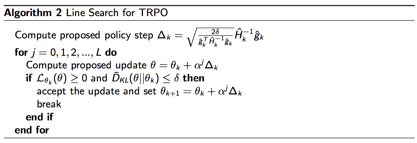
\[\begin{aligned} &\text{KL constraint:} \qquad \frac{1}{2}\,(\alpha \mathbf g_N)^\top \mathbf F(\theta_{\mathrm{old}}) (\alpha \mathbf g_N) = \varepsilon \\[8pt] &\theta_{\mathrm{new}} = \theta_{\mathrm{old}} + \alpha\,\mathbf g_N \\[12pt] &\alpha = \sqrt{ \frac{2\varepsilon} {\mathbf g_N^\top \mathbf F(\theta_{\mathrm{old}})\mathbf g_N} } \\[12pt] &\theta_{\mathrm{new}} = \theta_{\mathrm{old}} + \sqrt{ \frac{2\varepsilon} {\mathbf g_N^\top \mathbf F(\theta_{\mathrm{old}})\mathbf g_N} } \; \mathbf F(\theta_{\mathrm{old}})^{-1} \nabla_\theta U(\theta)\Big|_{\theta=\theta_{\mathrm{old}}} \end{aligned}\]

Line Search For TRPO

Because the quadratic KL approximation is in the end just an approximation that is done with neural nets, the actual KL may not actually be \(\leq \epsilon\) like we want it. Instead we try something that just tests different step sizes \(\alpha^{j+1} = c\,\alpha^j\) with a shrink factor \(c \in (0,1)\) to gauge a KL constraint that works and a positive surrogate improvement.