VAEs are a specific form of autoencoders. However, they differ in that they are probabilistic models that encode latent variables of training data as a probability distribution, not a singular output. They are generative models, because they are probabilistic: we sample latent vectors from the distribution and decode it for output. The name variational comes from Variational Inference.

VAE Scenario

Our vanilla autoencoders are purely for learning a useful latent representation - but we have no way of sampling useful $z$ latent vectors for proper generation. Hence VAEs solve the problem by conditioning our autoencoders to learn continuous and structured latent spaces, giving as an actual tool for image generation tasks!

By continuous, we mean small perturbations in latent space should generate a small change in decoder output. Structure means different vectors in latent space can give us semantic meaning!

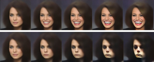
The smile vector, trained on the CelebA dataset with VAEs

VAE Overview

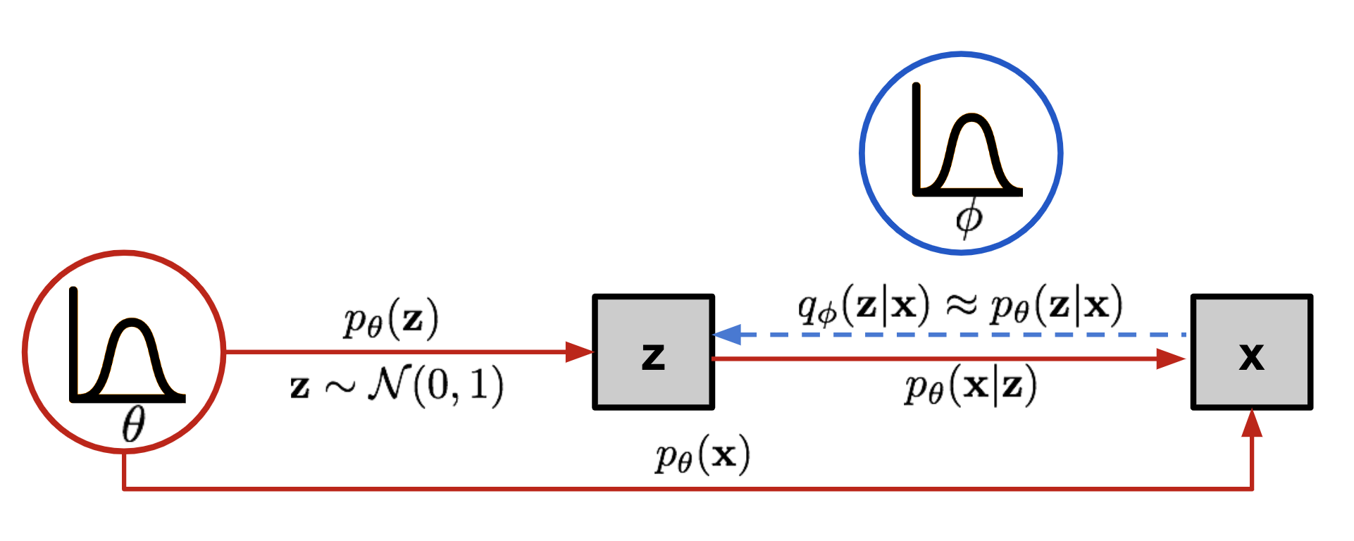
Let $\theta$ define the parameters of our VAE model. Then we describe the relations between our input data $x$ and latent vector $z$ as

our prior $p(z)$ defines a known distribution for sampling latent vectors, to which then we can pass through our decoder for image generation
our true likelihood $p_{\theta}(x \mid z)$ which is our decoder! For a specific image $x^i$, there is a specific region of $z$ in our prior distribution that has high probability of reconstructing $x^i$ with our decoder: this is what contributes to the integral for $p_\theta(x) = \int p_\theta(x\mid z)\,p(z)\,dz$ - where $p_{\theta}(x \mid z)$ has the most mass and $p(z)$ is large. Remember that during inference for actual random generation, we randomly sample from $p(z)$ and pass it through our decoder $p_{\theta}(x \mid z)$ for a new random image. Encoder is not needed there.
our true posterior $p_{\theta}(z \mid x)$ By Baye’s Rule, $p_\theta(z\mid x) = \frac{p_\theta(x\mid z)\,p(z)}{p_\theta(x)}.$ This is intractable for the reasons above, and must be approximated, through network parameterized by $\phi$ instead!
our approximate/variational posterior $q_{\phi}(z \mid x)$ which is our encoder! We need a good encoder $q_{\phi}(z\mid x)$ that generates a region of $z \sim q_{\phi}(z\mid x)$ (and later which decodes to good enough $x$).
our marginalized likelihood $p_{\theta}(x)$ or evidence of observing $x$ under our VAE model - our goal for MLE! $p_\theta(x) = \int p_\theta(x\mid z)\,p(z)\,dz$ We need this for our likelihood function and determining loss. And we can try sampling $z$ from our prior running through our decoder to produce sample estimates of our marginal for using in Monte Carlo sampling, but this will also be a bad approximation. We can never exactly compute this distribution and hence it is intractable.

Aside: Generative Modelling Assumptions

Review of Deep Generative Learning

The whole goal of deep generative modeling is to learn a model of the complex manifold of the data distribution of images so that the probability of observing images in our original data distribution is high in our learned model.

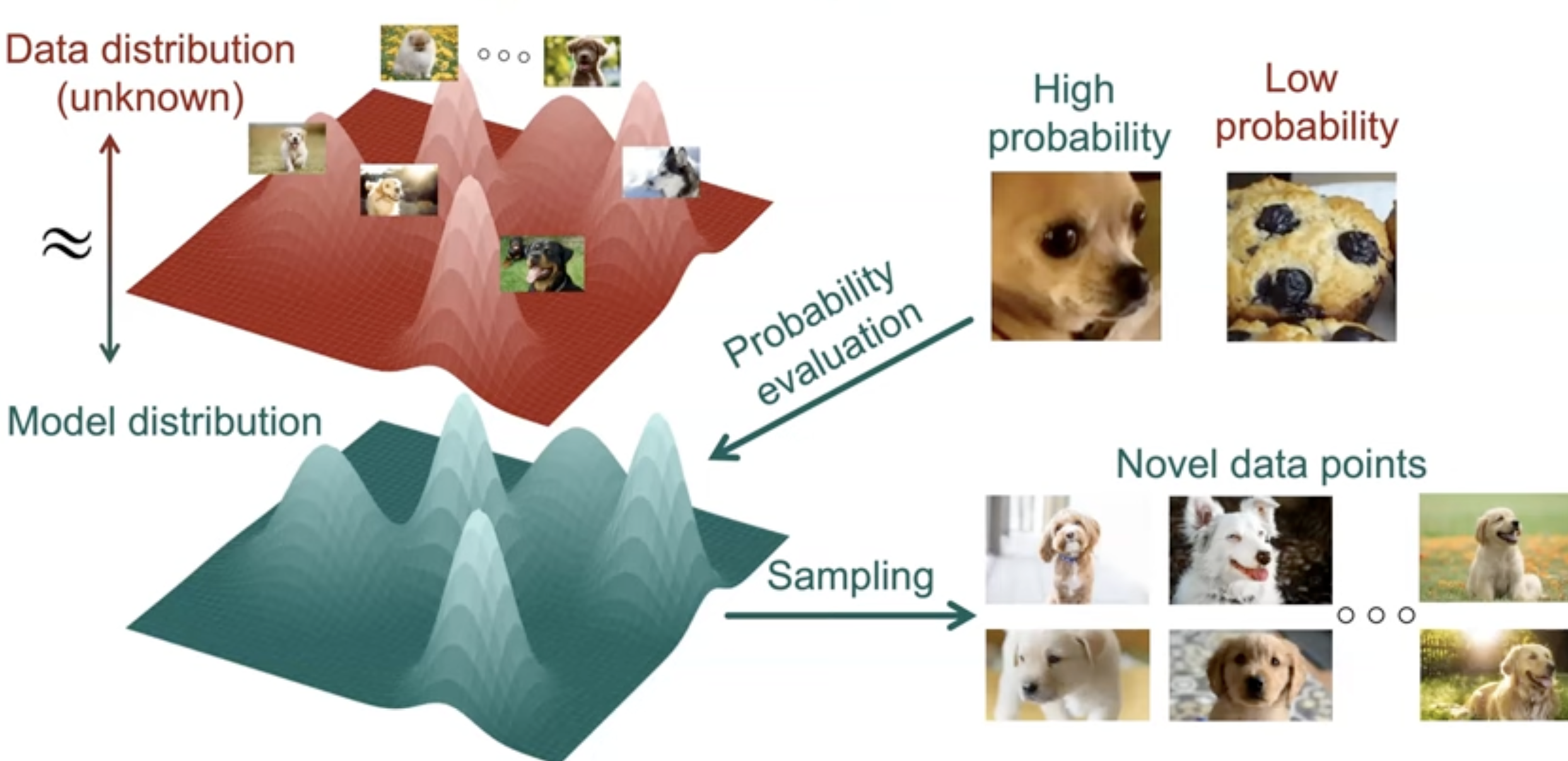
For VAEs, this is done specifically by modeling specifically the mapping from a gaussian prior to data distribution as best as possible through our decoder model.

Gaussian Distribution for Generative Models

One interesting caveat almost anyone would ask is - why are gaussian distributions so commonly used in generative modeling?

Convenient mathematic properties
- The KL Divergence between 2 gaussians is easy to compute - we do not require monte carlo sampling to estimate an expectation if an analytic form exists. Outside of VAEs this can be seen as a property that would be convenient in loss formulations for may use cases.
- The linear combination of many gaussians is also a gaussian. This is a property very convenient for the forward process of diffusion models.
- The closed form density being simple allowing nice simplifications in any derivation
Among all continuous distributions with a fixed mean and variance, the Gaussian has the largest entropy Intuitively, this means is that the latent prior is the most “uninformative” and the learned assumptions/patterns are maximally embedded within the encoder/decoder models that are actually used for image generation! Both the encoder/decoder models are learned to transform the simple gaussian into a complex distribution modeling our data distribution of images.

Reason 2 is great intuition, but in practice, any probability distribution can be used. It was shown in Cold Diffusion - Inverting Arbitrary Image Transforms Without Noise, that different types of noise transformations for diffusion-style image generation also work well. I think that the main reason is surely then number 1. It’s the most well studied distribution due to its simplicity and how common it is because of the Central Limit Theorem.

Encoder

In order to sample our latent variable $z \sim \mathbb{R}^J$, we define it as sampling from a prior distribution we know such as the Gaussian distribution

\[\boldsymbol{z} \sim \mathcal{N}(\boldsymbol{0}, \boldsymbol{I})\]

Because our posterior for the latent (inference) is intractable

\[\begin{align} p_{\theta}(z \mid x) &= \frac{p_{\theta}(x \mid z)p(z)}{p_{\theta}(x)} \tag{Baye's Rule}\\ &= \frac{p_{\theta}(x \mid z)p(z)}{\int_{z} p_{\theta}(z,x) dx} = \frac{p_{\theta}(x \mid z)p(z)}{ \int_{z} p_{\theta}(z) \cdot p_{\theta}(x \mid z) dz} \tag{Law Total Probability} \end{align}\]

then we approximate using variational inference, using our approximate posterior encoder $q_{\phi}(z \mid x)$ which outputs $\mu_{\phi}(x)$ and $\sigma_{\phi}^2(x)$ in order to describe a gaussian distribution. Note that our variational family need not be gaussian!, but we like for it to be because of easy parametrization and simplicity reasons.

\[q_\phi(z \mid x) = \mathcal N\big(z; \mu_\phi(x), \operatorname{diag}(\sigma_\phi^2))\]

Reparameterization Trick

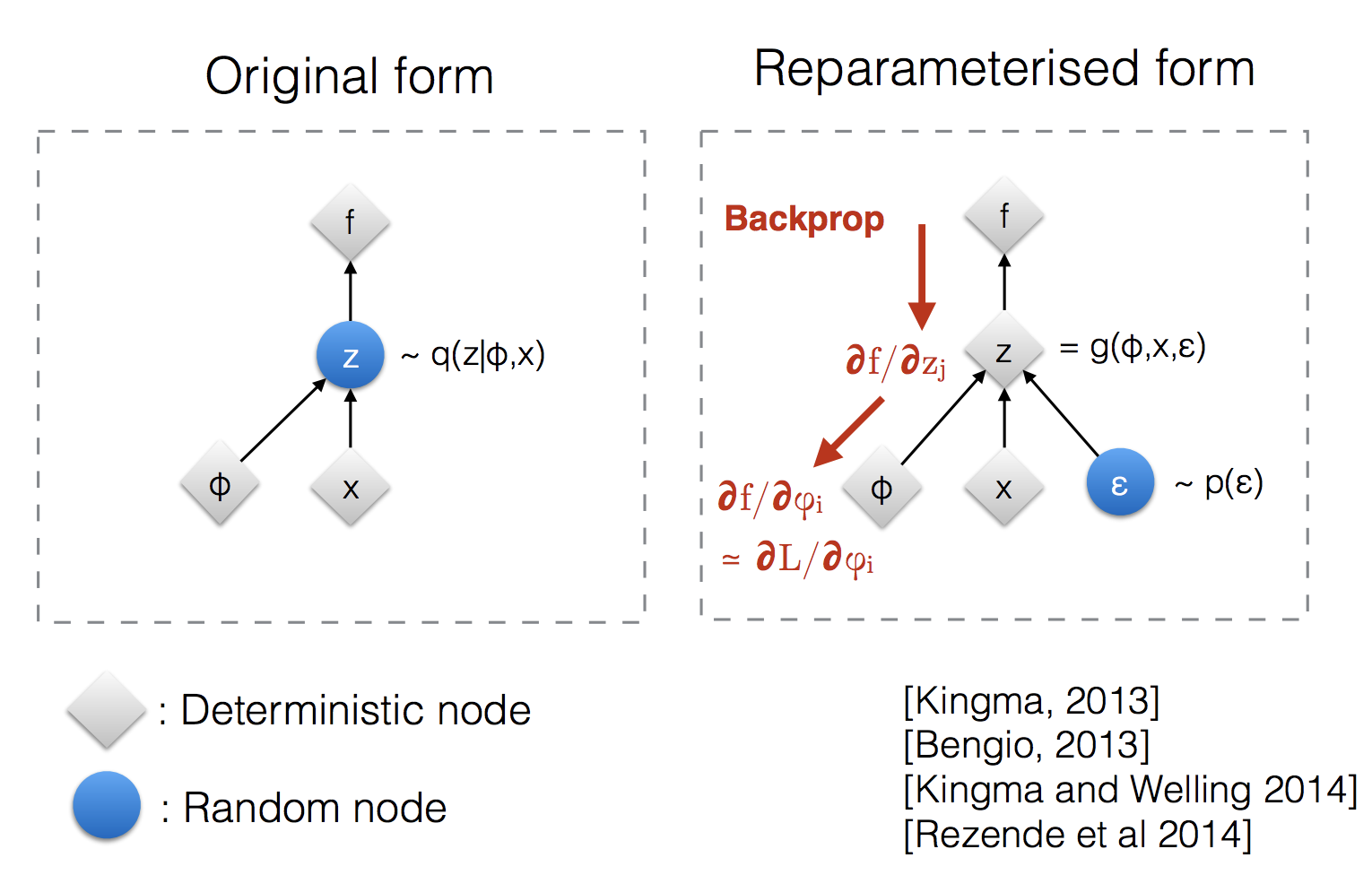
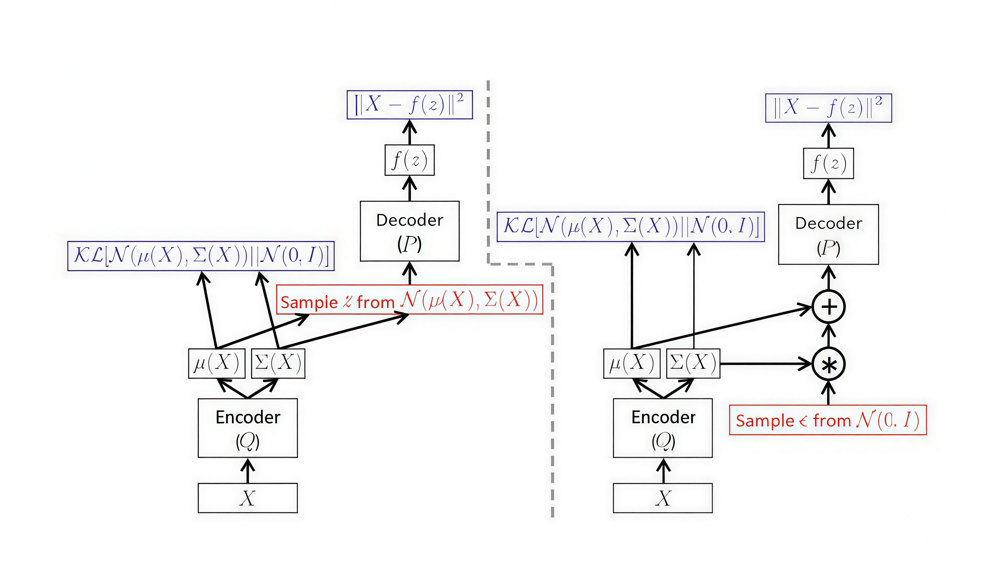
Instead of sampling $z$ from $q_\phi(z\mid x)$ directly, in order for gradients to actually flow from $z$, then we must reparameterize $z$ as

\[z = \mu_\phi(x) + \sigma_\phi(x)\odot \varepsilon,\ \varepsilon \sim \mathcal{N}(0, I)\]

Now the computation of $z$ is deterministic, with the randomness is offloaded to $\epsilon$

In our computation graph, we see that the computation graph is back propagable!

Now, fully our VAE can be shown as

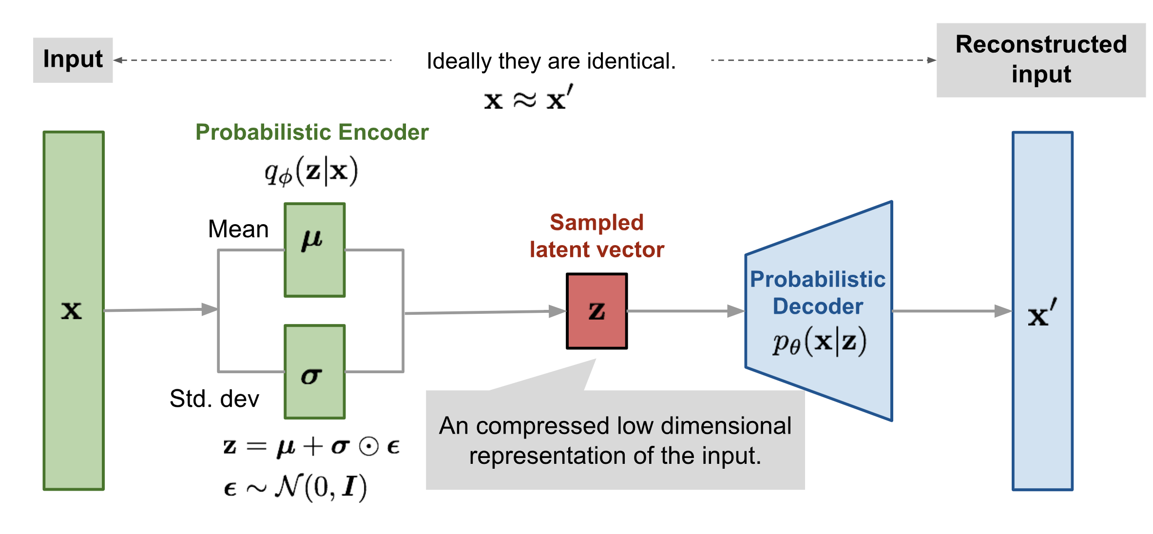
Decoder

We also can model the decoder $p_{\theta}(x \mid z)$ for generation as a gaussian (for real-valued data vs binary? !REVIEW)

\[x \sim \mathcal{N}(f_{\theta}(z), \sigma)\]

where $f_{\theta}(z)$ is our deterministic neural net part of the decoder. Again for sampling we also need to use the reparameterization trick as discussed before.

Loss Function - VAE Training Objective

This is the most important and complex part in understanding VAEs!

MLE

For a review of MLE, remember the goal in MLE is to find the optimal $\theta^*$ such that $p_{\theta}(x \mid z),\ p_{\theta}(z)$ best explain our dataset $X=\{x^{(i)}\}_{i=0}^N$ using the likelihood estimation of our marginalized likelihood $p_{\theta}(x)$ for all training samples in our VAE.

\[\theta^*=\underset{ \theta }{ \arg \max } \prod_{i=0}^{N} p_{\theta}(x^i)\]

or more simply log likelihood.

\[\theta^*=\underset{\theta}{\operatorname{arg max}} \sum^{i=N}_{i=0} \log p_\theta (x^{(i)})\]

But remember, that this inner term is something intractable.

\[p_\theta(\mathbf{x})= \displaystyle \int_{z}p_\theta(\mathbf{z})p_\theta(\mathbf{x}\vert \mathbf{z})dz\]

But this is where the magic of ELBO comes in

Deriving the ELBO, Evidence Lower Bound

By evidence, we can derive the log likelihood of a function given fixed parameters $\theta$. The derivation is a bit tricky, 1. we need to introduce an expectation somehow to introduce KL divergence terms 2. the identity multiplication in the log term is needed to give us tractable terms; using Jensen’s Inequality there are other derivations that turn out simpler. Since the term is intractable, we do some manipulation

For a single sample $x$, then this resolves to

\[\begin{flalign} &\log p_{\theta}(x) \tag{log likelihood}\\ = &\mathbb{E}_{z \sim q_{\phi}(z \mid x)} [\log p_{\theta}(x)] \tag{$ {\mathbb{E}_\text{distr.}}[Constant] = Constant$}\\ = &\mathbb{E}_{z \sim q_{\phi}(z \mid x)}\left[ \log \frac{p_{\theta}(x \mid z)p_{\theta}(z)}{p_{\theta}(z\mid x)} \right] \tag{$p_{\theta}(z \mid x) = \frac{p_{\theta}(x \mid z)p_{\theta}(z)}{p_{\theta}(x)}$ (Bayes Rule)}\\ = &\mathbb{E}_{z \sim q_{\phi}(z \mid x)}\left[ \log \frac{p_{\theta}(x \mid z)p_{\theta}(z)}{p_{\theta}(z\mid x)} \frac{q_{\phi}(z \mid x)}{q_{\phi}(z \mid x)} \right] \tag{Identity}\\ = &\mathbb{E}_{z \sim q_{\phi}(z \mid x)}\left[ \log p_{\theta}(x \mid z) \frac{p_{\theta}(z)}{q_{\phi}(z \mid x)} \frac{q_{\phi}(z \mid x)}{ p_{\theta}(z\mid x) } \right] \tag{Rearranging below}\\ = &\mathbb{E}_{z \sim q_{\phi}(z \mid x)}[\log p_{\theta}(x \mid z)] - \mathbb{E}_{z \sim q_{\phi}(z \mid x)}\left[\log \frac{q_{\phi}(z\mid x)}{p_{\theta}(z)} \right] + \mathbb{E}_{z \sim q_{\phi}(z \mid x)}\left[\log \frac{q_{\phi}(z \mid x)}{p_{\theta}(z\mid x)} \right] \tag{expand logs + L.O.E}\\ = &\underbrace{ \mathbb{E}_{z \sim q_{\phi}(z \mid x)}[\log p_{\theta}(x \mid z)] - D_{KL}(q_{\phi}(z\mid x) \parallel p_{\theta}(z)) }_{\text{ELBO (tractable)}} + \underbrace{ D_{KL}(q_{\phi}(z\mid x) \parallel p_{\theta}(z\mid x)) }_{ \geq 0 } \tag{$p_{\theta}(z\mid x)$ intractable! }\\ \geq &\underbrace{ \mathbb{E}_{z \sim q_{\phi}(z \mid x)}[\log p_{\theta}(x \mid z)] - D_{KL}(q_{\phi}(z\mid x) \parallel p_{\theta}(z)) }_{\text{ELBO!}} \tag{KL is always nonzero!} \end{flalign}\]

The last component $D_{KL} \left[ q_{\phi}(\mathbf{z}|\mathbf{x}) \parallel p(\mathbf{z}|\mathbf{x}) \right]$ measures the difference between our encoder estimate’s posterior and our real posterior (the basis of Variational Inference, since we don’t know what the real posterior is!) and is importantly not tractable. So it is important to realize the ELBO is only a lower bound, so we are not necessary always optimizing the log-likelihood. But generally, because this is the gap between the true log likelihood and our ELBO estimate, minimizing this term is beneficial for accurate estimates!

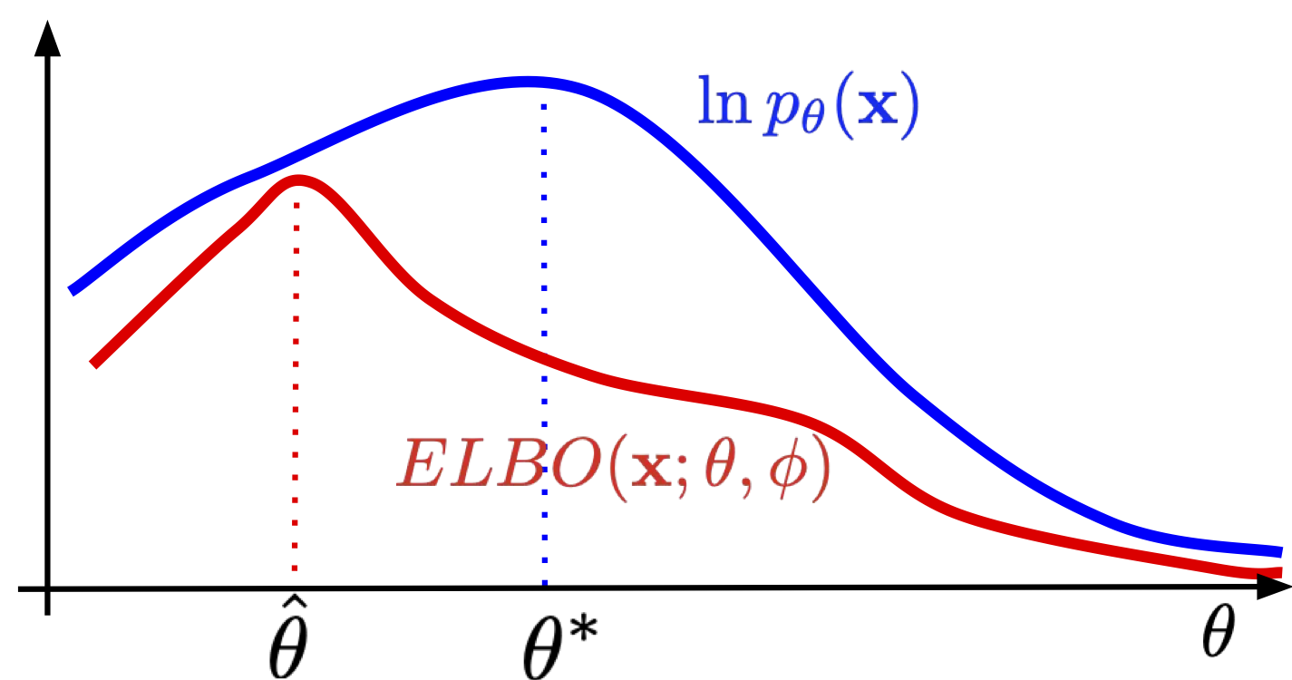
maximizing ELBO is not equivalent to maximizing log likelihood!

Taking a closer look at what maximizing the ELBO means (conventionally, this loss expression should be negated, but lets think about maximizing loss/ELBO for clarity).

\[\mathcal{L}\bigl(x^{(i)},\theta,\phi\bigr) = \underbrace{ \mathbb{E}_{z\sim q_\phi(z\mid x^{(i)})}\bigl[\log p_\theta(x^{(i)}\mid z)\bigr] }_{\text{Reconstruction Loss} } \;-\; \underbrace{ D_{\mathrm{KL}}\bigl(q_\phi(z\mid x^{(i)})\;\|\;p(z)\bigr) }_{\text{Regularization Term} }\;\]

Reconstruction loss in order to generate likely samples $x^i$. For each $z$ drawn from the encoder’s approximate posterior, how likely can we generate that sample $x^i$?
Regularization term in order to push the encoder (approximate posterior) to match our gaussian prior. We encourage the approximate posteriors to fit in a large gaussian, so that $\mu_\phi(x)$ is somewhat near the origin.
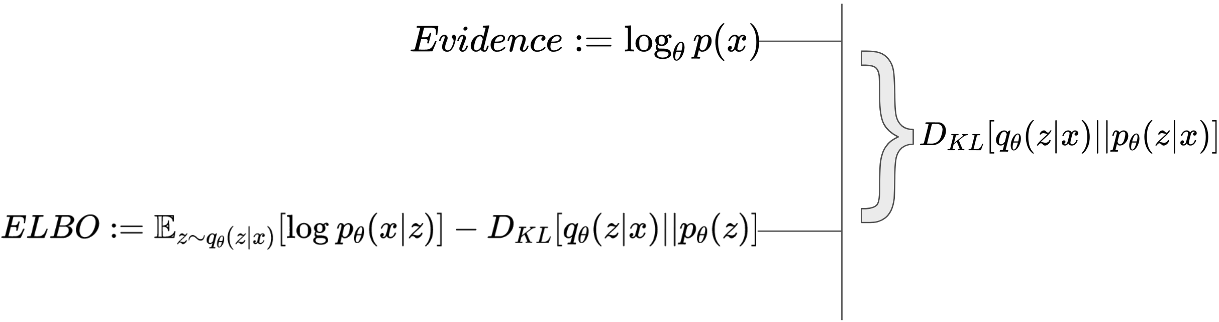
Illustration of ELBO term and regularization
With a gaussian prior, this expression has closed form:

\[D_{\mathrm{KL}}(q_\phi(z\mid x)\,\|\,p(z)) = \frac{1}{2}\sum_j \Big(\mu_j(x)^2 + \sigma_j(x)^2 - \log \sigma_j(x) -1 \Big)\]

Note then we prevent “spikes” from forming (low variance posteriors)

As for actually computing the terms

This requires drawing $K$ samples of $z$.

\[\mathbb{E} _{z \sim q_\phi(z \mid x)} [\log p_\theta (x \mid z)] \approx \frac 1 K \sum_k \log p_\theta(x \mid z^{(k)})\]

For the log term also being Gaussian, this is actually equivalent to MSE loss or minimizing $\|x^{(i)} - f_\theta(z)\|^2,$
Since we have a closed form analytical expression as above, then all we need to do is for each sample $x^{(i)}$ run it through the encoder and calculate the KL loss for that sample.

Log-Likelihood

So we aim to minimize negative log-likelihood which we can do using our empirical average.

\[\mathcal{L}(x; \theta, \phi) = - \frac{1}{N }\sum_{i=1}^N \log p_\theta(x_i) = - \frac{1}{N} \sum_{i=1}^N \text{ELBO}(x_{i}) = - \frac{1}{N} \sum_{i=1}^N \log p_{\theta}(x \mid z^{(i)}) - D_{KL}(q_{\phi}(z\mid x) \parallel p(z))\]

Training VAEs

Feed a data point $x$ to encoder to predict $\mu_{\phi}(x)$ and $\sigma_{\phi}^2(x)$
Sample a latent variable $z$ from $q_{\phi}(z \mid x) = \mathcal{N}(z; \mu_{\phi}(x), \sigma_{\phi}^2(x))$
Feed $z$ through decoder to predict $\hat{x} = q_{\theta}(x \mid z)$
Back propagate negative ELBO

Readings

Many of these require higher degree of mathematical maturity or a depth that may be overkill

https://lilianweng.github.io/posts/2018-08-12-vae/#reparameterization-trick https://mbernste.github.io/posts/vae/ https://jmtomczak.github.io/blog/4/4_VAE.html https://yonigottesman.github.io/2023/03/11/vae.html https://gaussian37.github.io/deep-learning-chollet-8-4/