Evolutionary Methods in Reinforcement Learning

Evolutionary Search as Black-Box Policy Optimization

These are called evolutionary methods because they closely follow the evolution of a population!

Initialize a population of policy parameter vectors $\theta_{i}$ randomly aka Genotypes
Make random perturbations to each parameter vector $\theta_{i}'$ Simulating mutations in offspring
Evaluate the perturbed parameter vector along some fitness function $F(\theta_{i}')$ Survival of the fittest
Update your policy parameters to favor the best performing parameter vectors based on fitness score $F(\theta)$ Enabling fitness in this offspring

These are examples of black-box policy optimization, where we treat the policy and environment as a “black box” that we can query (run rollouts) and update our policy based purely on performance we can observe

we do not learned a structured “state” representation of state values and/or state-action values based on the structure of Bellman equations like in Value-Based Methods in Reinforcement Learning
use do not use analytic gradients of the return w.r.t. policy parameter $\theta$ directly (as in Policy Gradient Methods in Reinforcement Learning). Methods like NES may do so indirectly, where we compute gradients w.r.t the parameters $\phi$ of a search distribution that $\theta$ is drawn from. There is subtle, but huge difference!

CEM: Cross-Entropy Method

In this method we consider policy parameters sampled from a isotropic Gaussian matrix:

Initialize a search distribution $p_{\phi}(\theta)$ where $\mu=0$ and $\Sigma = 100I$

Repeat for $k$ steps:

sample $n$ policy parameters $\{ \theta_{i} \}_{i=1}^n$ from current multivariate Gaussian distribution matrix
Evaluate those $n$ parameters averaged over $L$ rollouts to generate a reward signal or scalar return $F(\theta_{i})$
select a proportion $\rho$ of those parameters with highest score as our $\lfloor \rho n \rfloor$ elite samples!
use their corresponding $\mu$ and $\sigma^2$ to update our reference matrix for sampling, which basically means setting the new mean as the mean of those highest $\lfloor \rho n \rfloor$ parameters and setting the new variance as simply the variance of those selected elite samples!

\[\begin{align} \\ & \mu \in \mathbb{R}^k ,\forall j \in [k]\\ & \mu(j) = \frac{1}{\lfloor \rho n \rfloor}\sum_{i=1}^{\lfloor \rho n \rfloor}\theta'_i(j) \\ & \sigma^2(j) = \frac{1}{\lfloor \rho n \rfloor}\sum_{i=1}^{\lfloor \rho n \rfloor} (\theta'_i(j) - \mu(j))^2 + \eta \end{align}\]

This worked really well up to the 2010’s and in low dimensional search space dimensions, shown to work well in Tetris (Szita, 2006), where we can craft a value function that is a linear combination of 22 basis functions $\phi(s)$ (individual column heights, height differences, etc)

\[V_{w}(s) = \sum_{i=1}^{22} w_{i} \phi_{i}(s)\]

and execute CEM on the weight vector $w$, evaluating fitness score based on the mean reward that weight matrix gives when computing a policy based on $V_{w}(s)$!

These evolutionary search methods weren’t a threat to DQN implementations at the time because they couldn’t scale to large non-linear neural nets with thousands of parameters. The fact that we rely on random sampling to somehow perturb each dimension of the weights to the optimal direction isn’t really sample-inefficient in very high dimensions - what if $w \in \mathbb{R}^{10^{9}}$?

Variants like CMA-ES, NES, and OpenAI’s scalable ES method make iterative improvements on CEM - but there is a reason why modern policy optimization methods use the information of a gradient vector in order to realize the best policy as we will see in policy gradient methods later on.

CMA-ES: Covariance Matrix Adaptation

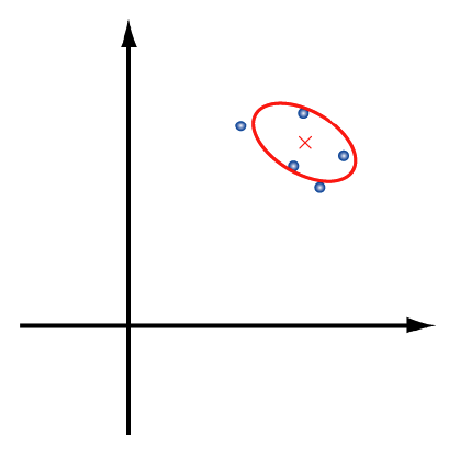
Instead of limiting ourselves to diagonal Gaussian, we search by learning a full covariance matrix so instead of just updating the mean and variances, we’re updating the entire matrix.

Imagine our samples are in 2-D dimension. Then visually, if there is an objective function we are trying to reach that is best maximized with samples spread in the shape 2d rotated ellipse, then we should utilize all the entries in a full covariance matrix which rotates a standard diagonal gaussian matrix (x-y aligned ellipse) to best maximize this objective function efficiently.

Our mean update can also be either a) iterative - as a weighted step from $\mu_{t}$ towards the elites or b) a simple weighted recombination of the elites

\[\mu_{t+1} = \mu_t + \alpha \sum_{i=1}^{n_{\text{elit}}} w_i\left(\theta^{\text{elit},t}_i - \mu_t\right) \text{ or } \mu_{t+1}=\sum_{i=1}^{n_{\text{elit}}} w_i \theta^{\text{elit},t}_i\]
Our covariance update now updates the covariance of the Gaussian search distribution to match the spread and correlations of the current elite set! We add a regularizer to prevent the variance from prematurely collapsing to $0$ too quickly

\[\Sigma_{t+1} = \mathrm{Cov}(\theta^{\text{elit},t}_1,\theta^{\text{elit},t}_2,\ldots) + \epsilon I\]

NES - Natural Evolutionary Strategies

NES optimizes our expected fitness objective by updating the parameters of our search distribution through a natural gradient, specifically updating our learned mean $\mu$, while fixing our covariance this time. NES considers every offspring when updating our policy parameters, because when deriving this gradient, we get an expectation term that has to be approximated with Monte-Carlo sampling.

Consider the parameters of our policy $\theta \in \mathbb{R}^d$ are sampled from a Gaussian distribution with learned mean $\mu \in \mathbb{R}^d$ and fixed diagonal covariance matrix $\sigma^2I$ (which is not being learned). We denote this search distribution as $P_{\mu}(\theta)$

\[\theta \sim P_{\mu}(\theta ) = \mathcal{N}(\mathbf{\mu}, \sigma^2 I)\]

Our goal is find the best possible search distribution, parameterized by $\mu$, that our policy is sampled from (through $\theta$)

\[\max_{\mu} \mathbb{E}_{P_{\mu}(\theta)}[F(\theta)]\]

based on a fitness score which is the expectation of reward over entire trajectories

\[F(\theta) = \mathbb{E}_{\tau \sim \pi_{\theta},\ s_{0} \sim \mu_{0}(s)}[R(\tau)]\]

Our goal is to derive a gradient update for $\mu$, so that we can apply a gradient ascent optimization process to find the optimal $\mu$!

Deriving the gradient estimator

Computing the update for our mean $\mu$ through this objective is as follows:

\[\begin{flalign} \nabla_{\mu} \mathbb{E}_{\theta \sim P_{\mu}(\theta)}[ F(\theta)] &= \nabla_{\mu} \int P_{\mu}(\theta) F(\theta) d\theta \tag{use pdf to integrate out expectation}\\ = \int \nabla _{\mu} P_{\mu} (\theta) F(\theta) d\theta &= \int P_{\mu}(\theta) \frac{ \nabla_{\mu} P_{\mu}(\theta)}{P_{\mu}(\theta)} F(\theta) d\theta\\ &= \int P_{\mu}(\theta) \nabla_{\mu} \log P_{\mu}(\theta) F(\theta) d\theta \tag{derivative of log trick!} \\ &= \mathbb{E}_{\theta \sim P_{\mu}(\theta)}[ \nabla_{\mu} \log P_{\mu}(\theta) F(\theta)] \tag{based on pdf}\\ &\approx \frac{1}{N}\sum_{i=1}^N \nabla_\mu \log P_\mu(\theta_i)\,F(\theta_i) \tag{Monte Carlo Sampling}\\ &\approx \frac{1}{N}\sum_{i=1}^N \frac{\theta_i-\mu}{\sigma^2} F(\theta_{i}) \tag{$\log P_{\mu}(\theta) = - \frac{\parallel \theta - \mu \parallel^2}{2\sigma^2} + const.$ for diagonal Gaussians}\\ &\approx \frac{1}{N}\sum_{i=1}^N \frac{\epsilon_i}{\sigma}\,F(\mu+\sigma \epsilon_i) \tag{Reparameterization trick for $\theta$} \end{flalign}\]

We really need to justify the intuition for why we use the log-probability trick: The point is we need to estimate the gradient using Monte-Carlo sampling, but to do that we need the pdf within the integral to convert to an expectation - when otherwise we just have $\nabla_{\mu}P_{\mu}(\theta)$ !

To expand on that last step, in order to back propagate through Gaussian distributions to $\mu$, then the sampling of $\theta_{i} \sim \mathcal{N}(\mu, \sigma^2 I)$ needs to be converted through the reparameterization trick so that $\theta_{i} = \mu + \sigma \epsilon_{i},\ \epsilon_{i} \sim \mathcal{N}(0, I)$.

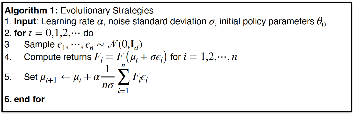
From this derivation, we have shown that this gradient to update the mean $\mu$ can be estimated by

sampling $N$ parameters $\theta_{i}$, running trajectories for each parameter, and obtaining our scalar fitness score $F(\theta_{i})$ for each sample
Then we simply need to scale by a sampled noise term $\epsilon$ divided by our variance $\sigma$ and average out all scaled terms!

Based on this derivation we can now apply gradient ascent to iteratively update our $\mu$! (based on learning rate $\alpha$)

\[\mu_{t+1} = \mu_{t} + \alpha \left[ \frac{1}{n \sigma} \sum_{i=1}^n \epsilon_{i} F(\theta_{i}) \right]\]

Black-Box Optimization

To clarify, this is still black-box optimization:

We do not need to know anything about how we are computing our fitness score, we simply realize raw output returns given our samples $\theta_{i}$
We are not computing computing analytic gradients of $F(\theta)$ wrt to $\theta$ in order to update our policy parameters directly; in fact, we compute gradients wrt to a different, known object that we have set: the search distribution probability density $P_{\mu}(\theta)$

Scalability + Parallelization of ES

!REVISIT The reason why we can scale NES well for large dimension of policy parameters $\theta$ when we are working with large policy networks is that we can parallelize the fitness score for each sampled $\theta_{i}$ for a corresponding worker process, where each worker can individually compute this term $\epsilon_{i} F_{i}(\theta_{i})$.

A bottleneck however, would be naively sending back and forth this large $\theta_{i} = \mu_{t} + \sigma \epsilon_{i}$ vector across all our $n$ workers:

Coordinator broadcasts $\mu_{t}$ once per update step to all workers
Coordinator sends $\epsilon_{i}$ to all $n$ workers individually, which allows every worker to compute $\theta_{i}$
Each workers runs trajectories and sends back $F(\theta_{i})$ to every other worker

Because of reparameterization only this $\epsilon_{i}$ needs to be sent to all $n$ workers, but this is still a very large parameter, so instead in a 2017 OpenAI paper, we use a pseudo random number generator to compute $n$ (tiny) seeds and then send these known small seeds to the $n$ workers, which can they reconstruct each large dimension $\epsilon_{i}$ and compute our returns $F(\theta_{i})$ which is just a scalar! So communication time is cut a lot.

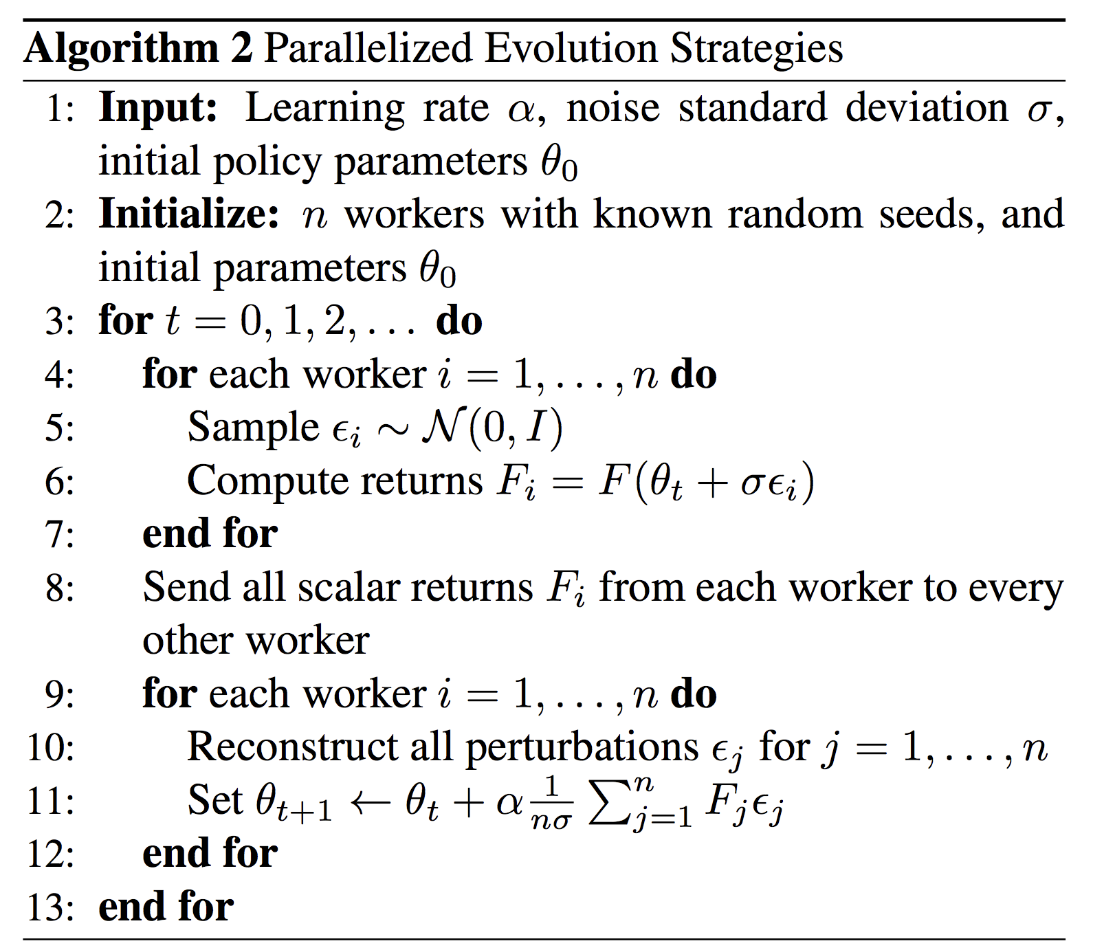
Note that here the current policy parameters $\theta_{t}$ are the center/mean of the perturbation distribution $\mu_{t}$

Local Maxima Issue

ES methods can easily get stuck in local optima. In order to prevent ES methods from getting stuck in local optima, we average fitness scores across

multiple tasks
related environments so that the search is biased towards policy parameters that are robust to variations of task/environment similar the original set and not exploit local maxima in the original task/environment.