published 2026-01-01·created 2025-12-31·updated 2026-09-10
Motivation
Given a dataset sampled from an unknown data distribution, we want to learn how to generate new samples from that distribution. While originally applied to image generation to replace GANs, this applies to
video generation
music synthesis
molecule generation
galaxy generation and astrophysical simulations
generative visuomotor policies in roboticic manipulation (modeling the conditional distribution of actions given observation embeddings)
Setup
How do we model distributions? One one hand, we can define modeling distributions by defining a flexible function \(\phi(x)\) yielding a density of \(p(x) = \frac{\phi (x)}{Z}\) where \(Z\) is a normalization constant. But this flexible definition makes computing \(Z\) difficult. On the opposing spectrum, we can define a non-flexible but easily tractable distribution such as mixture of gaussians, that may be easy to evaluate by are not capable to describe the structure of the complex data we are trying to model. Diffusion aims to be both 1. tractable and 2. flexible (apt to model any complex distribution).
The tractability comes from defining a Markovian chain that converts a simple known distribution (a Gaussian) to a target data distribution at the endpoint of this Markovian chain. Each step in the chain can be modeled by small and tractable perturbations (originally chosen to be gaussian noise. Empirically, it was discovered these perturbations can be arbitrary) “Since a diffusion process exists for any smooth target distribution, this method can capture data distributions of arbitrary form.”
Forward Diffusion Process: Markov Chain
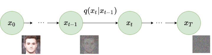
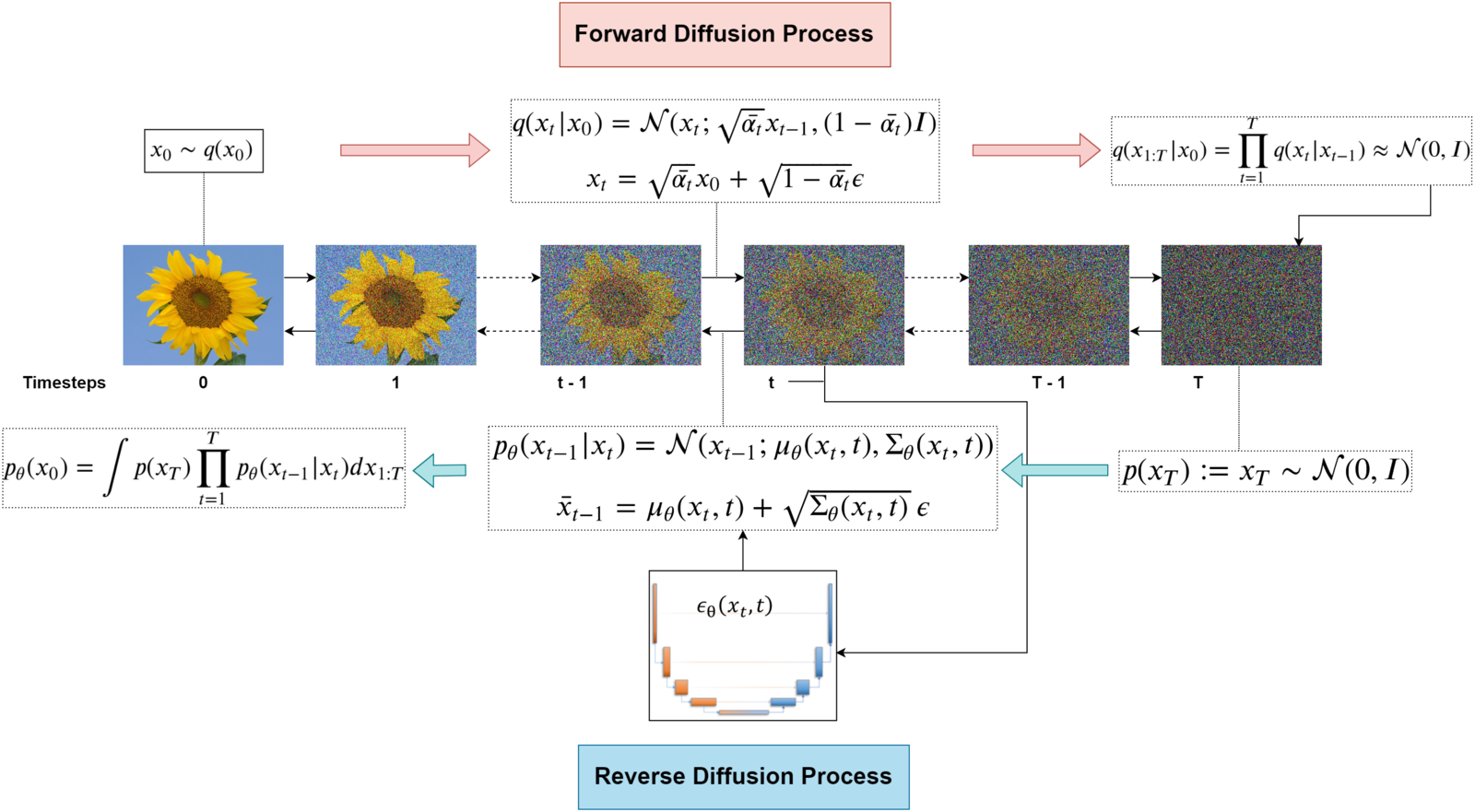
Given an image data point \(x_0\) sampled from the image dataset distribution \(x_0 \sim q(x)\), the forward process add gaussian noise in a series of \(T\) time steps, producing a sequence of noisy points at different timesteps (\(x_1, \dots x_T\)).
(In context of images, an image of \(d\) pixels can be flattened to a vector \(\in \mathbb{R}^d\) (or type-checking purposes image can be normalized into pixel intensities \([-1, 1]\) instead of \([0, 255]\)).
Each transition step is a conditional probability distribution (\(q(x_t \mid x_{t-1}): \mathbb{R}^d \rightarrow \mathbb{R}^+\)), giving us the probability density for the image \(x_t\) given the previous time step’s \(x_{t-1}\). We call this process Markovian, because it satisfies the Markov Property: each step only relies on the previous step: formally \(q(x_t \mid x_{0:t-1}) = q(x_t \mid x_{t-1})\).
\(\beta_t \in [0, 1]\) is a constant given from our noise scheduler, \((\beta_1, \beta_2, \dots, \beta_T)\) specifying the variance (noise intensity) added each time step.
Choice of Markovian Kernel?
We choose \(\sqrt{1-\beta_{t} }\) and \(\sqrt{ \beta_{t} }\) as multipliers because variances scale with the square of a multiplier. According to the reparameterization trick, since \(x_{t} = \sqrt{ 1-\beta_{t} } x_{t-1} + \sqrt{\beta_{t}} \epsilon\), and because \(x_{t-1}\) and \(\epsilon\) are sampled independently, then
Since we normalized our image to \([-1, 1]\), \(var(x_0) \leq 1\) , so then \(\forall t,\ Cov(x_{t}) \leq I\). This property is called “variance preserving” in order to prevent variance from exploding through the entire forward process!
The more precise claim is that the second moment is preserved
Variance/Noise Schedule
Originally, the authors of DDPM utilizes a linear schedule.
Variance Schedule of Linear (top) vs Cosine (bottom)
Shortening the Forward Kernel
The joint distribution of the entire trajectory of \(T\) time steps is the product of all \(T\) different PDF
can be expressed a simpler closed form expression. Let’s define additional variables
\(\alpha_t = 1-\beta_t,\quad t=1,\dots,T\) defining “fraction” of the previous step’s signal retained
\(\bar\alpha_t = \prod_{s=1}^t \alpha_{s}\) denoting the “fraction” of the original image “left” after \(t\) time steps.
\(\epsilon_0, \dots, \epsilon_{t-1} \sim \mathcal{N}(0, I),\ \epsilon_i \in \mathbb{R}^d\) is the gaussian noise added at each time step
and induct on \(t\) or \(x_t\):
The key combined variance step is as follows: Since \(\epsilon_{t-2}\) and \(\epsilon_{t-1}\) are sampled independently, the linear combination of independent Gaussians stays Gaussian (with a combined mean of \(0\) still), and we can sum variance through linearity of variance.
As \(T \rightarrow \infty\), then we should have reached an isotropic Gaussian distribution, one where \(x_T \sim \mathcal{N}(0,I)\) follows a perfect gaussian distribution of mean \(0\). Note that is because \(\bar{\alpha}_{t} \rightarrow 0\) !
This is advantageous, because we all already know how to sample gaussian noise, so figuring out how to reverse the gaussian noise in the reverse diffusion process allows us to generate random images!
Reverse Diffusion Process
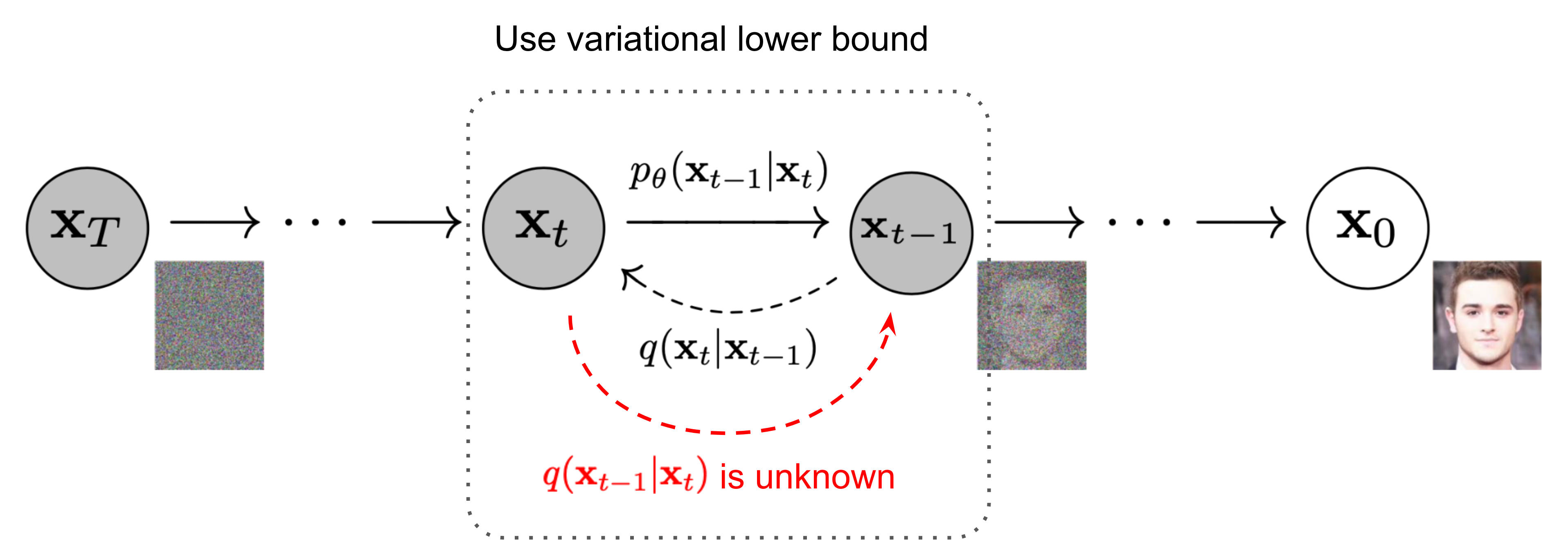
We want to learn the reverse distribution \(q(x_{t-1} \mid x_t)\) by learning a deep learning model \(p_{\theta}\) approximating this reverse distribution. This reverse process can generate new sample points from the data distribution using Gaussian samples as inputs. By iteratively applying the learned reverse transitions, we can generate samples approximating the data distribution.
But this exact reverse conditional \(q(x_{t-1}\mid x_{t})\) might not be Gaussian. In the small-step (continuous time limit), the reverse transition is locally approximately gaussian!, so we represent the reverse as a gaussian as well. So our model \(p_{\theta}\) is trying to estimate mean and variance:
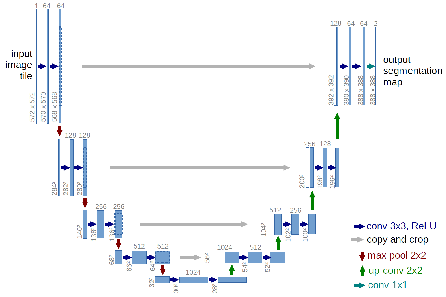
U-Net is a kind of neural network originally purposed for medical image segmentation (~2015) given the name based on the u-shape form when drawn:
In downsampling we operate on a feature extraction principle, applying 3x3 Convolutions followed by ReLu activation. Then iteratively apply a maxpool layer to reduce feature size while retaining features.
On the bottleneck layer, where most of the important features have been extracted it is processed even further
Then upsampling layer increases information using
skip connections to regain spatial details that may have been lost when downsampling.
we match a similar size region from downsampling, and copy a centered subset that matches width x height. Then we concatenate this to the channel dimension.
But the difficult is that, \(p_{\theta}(x_{0})^i\) requires marginalizing over all latent variables \(x_{1:T}\). Because we have \(T\) nested integrals this would be intractable to compute, so we can’t just optimize the log likelihood (marginal likelihood) directly.
We Since \(\log\) is a concave function, then Jensen’s Inequality (\(\log \mathbb{E} \geq \mathbb{E}[\log]\)) allows us to optimize an easier objective, the Evidence Lower BOund given by the inequality:
One perspective to view diffusion models is as a stack of \(T\) VAEs with an encoder encoding latents \(x_{1:T}\) and a decoder that decodes images closely matching \(x_{0}\).