We no longer consider black-box optimization methods. Instead of updating a search distribution $P(\theta)$ that our policy parameters are sampled from, we directly update our policy parameters $\theta$, using gradient estimates computed from sampled trajectories (policy gradients)! Then we search for a local maximum of a policy objective $U(\theta)$ by using gradient ascent.

Policy Objective

One reasonable policy objective is to maximize our expected trajectory reward over distribution of all trajectories parametrized by our policy parameters $\theta$ .

\[\begin{align} &\max_{\theta}. U(\theta) = \mathbb{E}_{\tau \sim P_{\theta}(\tau)}[R(\tau)] = \sum_{\tau}P_{\theta}(\tau) R(\tau) \tag{discrete trajectory space}\\ &R(\tau) = \sum_{t=0}^{T}\gamma^t r(s_t,a_t) \end{align}\]

Remember that $P_{\theta}(\tau)$ is the probability distribution over seeing that entire trajectory when we run $\pi_{\theta}$ in our environment which abstracts three key ingredients

the initial state being sampled from an initial state distribution
the dynamics of the environment resulting in stochastic next states $s_{t+1}$
the stochasticity of the policy in which actions are sampled from - this is what our $\theta$ actually parameterizes.

\[P_{\theta}(\tau) = \underbrace{ \rho_{0}(s_{0}) }_{ \text{initial state} } \prod_{t=0}^{T-1} \underbrace{ P(s_{t+1} \mid s_{t},\ a_{t}) }_{ \text{dynamics} } \underbrace{ \pi_\theta(a_{t} \mid s_{t}) }_{\text{action sampling}}\]

It’s assumed that $P_{\theta}(\tau)$ is a probability density function that is continuous and differentiable - necessary to propagate our gradient as we will see in the derivation: This really just means $\pi_\theta(a\mid s)$ is a policy that is differentiable.

Overview

Then the general structure of Policy Gradient Methods would follow something like

Initialize policy parameters $\theta$
Sample trajectories $\tau_{i} = \{ s_{t}^i, a_{t}^i \}_{t=0}^T$ by deploying the current policy $\pi_{\theta}(a_{t}\mid s_{t})$
Compute gradient vector $\nabla_{\theta} U(\theta)$ This is done through estimation from collected trajectories.
Apply a gradient ascent update $\theta \leftarrow \theta + \alpha \nabla _\theta U(\theta)$

We now need to figure out how to compute this gradient in order to find optimal $\theta$:

Aside: Finite-Difference Methods

One way to try and approximate policy gradient of $\nabla_\theta U(\theta)$ by nudging $\theta$ in every possible small amount dimension and approximate partial derivatives as such:

For each dimension $k \in [n]$ calculate the partial gradient

\[\frac{\partial U(\theta)}{\partial \theta_{k}} = \frac{U(\theta + \epsilon u_{k}) - U(\theta - \epsilon u_{k})}{2 \epsilon}\]

This was used to train these AIBO robots to run across a soccer field.

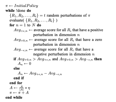
Policy Gradient Reinforcement Learning for Fast Quadrupedal Locomotion, Kohl and Stone, 2004

But this is really not feasible in high dimensions

Derivatives of the Policy Objective

Policy gradients aim to exploit our factorization of $P_{\theta}(\tau) = \prod_{t=0}^H P(s_{t+1} \mid s_{t}, a_{t}) \pi_{\theta}(a_{t} \mid s_{t})$ to compute approximate gradient estimate for

\[\nabla_{\theta} U(\theta) = \nabla _{\theta} \mathbb{E}_{\tau \sim P(\tau; \theta)}[R(\tau)]\]

In comparison to evolutionary methods, here the challenge is to compute derivatives w.r.t variables that parameterize a distribution that our expectation is summed over. The derivation uses the same log probability trick as derived for evolutionary methods; also we assume discrete trajectory space to sum over - if continuous, the derivation is largely the same.

\[\begin{flalign} \nabla_{\theta} \mathbb{E}_{{\tau \sim P_{\theta}(\tau)}}[R(\tau)] &= \nabla_{\theta} \sum_{\tau} P_{\theta}(\tau) R(\tau) \tag{expand expectation using pmf} \\ &= \sum_{\tau} \nabla_{\theta} P_{\theta}(\tau) R(\tau) \tag{sum rule} \\ &= \sum_{\tau} P_{\theta}(\tau) \frac{\nabla_{\theta} P_{\theta}(\tau)}{P_{\theta}(\tau)} R(\tau) \\ &= \sum_{\tau} P_{\theta}(\tau) [\nabla_{\theta}\log P_{\theta}(\tau)] R(\tau) \tag{log derivative trick} \\ &= \mathbb{E}_{_{\tau \sim P_{\theta}(\tau)}}[\nabla_{\theta} \log P_{\theta}(\tau) R(\tau)] \end{flalign}\]

The intuition is that our policy objective gradient is trying to

increase the log probability of trajectories that give a positive reward and
decrease the log probability of trajectories that give a negative reward.

The key observation is that this expectation can be simplified much further because our trajectories encapsulate the dynamics of the environment - but this is not specifically parametrized by our policy parameters, so the derivatives of our trajectories propagate further to specifically the derivatives of taking actions under our policy.

\[\begin{flalign} \nabla_{\theta} \log P_{\theta} (\tau)&= \nabla_{\theta} \log \left[ \rho(s_{0})\prod_{t=0}^T P(s_{t+1} \mid s_{t}, a_{t}) \pi_{\theta}(a_{t} \mid s_{t}) \right] \tag{factorizing our trajectory} \\ &= \nabla_{\theta} \left[\log \rho_{0}(s_{0}) + \sum_{t=0}^T \log P(s_{t+1} \mid s_{t}, a_{t}) + \log \pi_{\theta}(a_{t} \mid s_{t}) \right] \tag{using logs to sum out product!}\\ &= \nabla_{\theta} \left[ \sum_{t=0}^T \log \pi_{\theta}(a_{t} \mid s_{t}) \right] \tag{dynamics in env. are $\perp$ of policy parameters!} \\ &= \left[ \sum_{t=0}^T \nabla_{\theta} \log \pi_{\theta}(a_{t} \mid s_{t}) \right] \tag{sum rule} \\ \end{flalign}\]

Then completing our derivation:

\[\begin{flalign} \nabla_{\theta} \mathbb{E}_{\tau \sim P_{\theta}(\tau)}[R(\tau)] &= \mathbb{E}_{\tau \sim P_{\theta}(\tau)}[\nabla_{\theta} \log P_{\theta}(\tau) R(\tau)] \\ &= \mathbb{E}_{\tau \sim P_{\theta}(\tau)} [ \sum_{t=0}^T \nabla _{\theta} \log \pi_{\theta}(a_{t} \mid s_{t}) R(\tau)]\\ & \approx \boxed{\frac{1}{N} \sum_{i=1}^N \sum_{t=0}^T \nabla _{\theta} \log \pi_{\theta} (a_{t} \mid s_{t}) R(\tau) } \tag{Monte Carlo Estimation!} \end{flalign}\]

So to summarize when we compute our policy objective gradient, we use an empirical estimate from $N$ sampled trajectories!

\[\nabla_{\theta}U(\theta) \approx \hat{g} = \frac{1}{N} \sum_{i=1}^N \sum_{t=0}^T \nabla_{\theta} \log \pi_{\theta} (a_{t} \mid s_{t}) R(\tau)\]

Given this estimate, let’s try to interpret more this gradient estimate $\hat{g}$ is doing. During gradient ascent we update policy using $\theta \leftarrow \theta + \alpha \hat{g}$ . So along some sampled trajectory $\tau$ of all $N$ trajectories we have that

If $R(\tau)$ is high, then $\hat{g}$ is updating the policy $\theta$ to increase log-prob of taken action if it led to good return (because we move in the direction $\nabla_{\theta} \log \pi_{\theta}(a_{t}\mid s_{t})$
If $R(\tau)$ is bad along $\tau$, then $\hat{g}$ is updating the policy $\theta$ to decrease log-prob of taken action if it led to bad return

Computing Policy Gradient

And the natural question is whether the derivative term is computable - which yes it is.

If our action space is continuous, then our policy network can be gaussian, outputting a mean and standard deviation. If we want our policy to be deterministic, then the action would be simply the mean! So for multivariate gaussians (and for simplicity assume we are in the case where $\Sigma$ is fixed), then

\[\nabla_\theta \log \pi_\theta(a\mid s) = \left(\Sigma^{-1}(a-\mu_\theta(s))\right)^\top \nabla_\theta \mu_\theta(s)\]

where we can back propagate $\nabla_\theta \mu_\theta(s)$ through the mean part of the policy network.

What this looks like is:
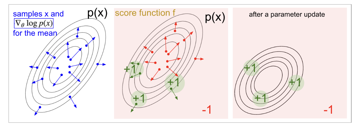
- Blue points are samples from the current Gaussian centered at $\mu$
- Each sample contributes a vector $\Sigma^{-1}(x^{(i)}-\mu)$ (points outward from the mean, scaled/rotated by $\Sigma^{-1}$)
- high-reward samples pull the mean toward themselves; low-reward samples push it away!
- Summing these gives an update direction that shifts $\mu$ to $\mu'$ favoring these high-reward actions
If our action space is discrete, obviously we apply a final softmax layer to output a discrete probability distribution over finite action space. Then if we want our policy to be stochastic, we can query a categorial distribution based on these probabilities for sampling. If we go through the derivation, in simple terms the update is “increase the logit of the chosen action” minus “the weighted averaged logit gradient under the current policy” which is as follows:

\[\begin{align*} \pi_\theta(a\mid s) &= \frac{e^{h_\theta(s,a)}}{\sum_b e^{h_\theta(s,b)}} \\ \log \pi_\theta(a\mid s) &= h_\theta(s,a) - \log\sum_b e^{h_\theta(s,b)} \\ \nabla_\theta \log \pi_\theta(a\mid s) &= \nabla_\theta h_\theta(s,a) - \nabla_\theta \log\sum_b e^{h_\theta(s,b)} \\ &= \nabla_\theta h_\theta(s,a) - \frac{1}{\sum_b e^{h_\theta(s,b)}} \nabla_\theta \sum_b e^{h_\theta(s,b)} \tag{chain rule}\\ &= \nabla_\theta h_\theta(s,a) - \frac{1}{\sum_b e^{h_\theta(s,b)}} \sum_b \nabla_\theta e^{h_\theta(s,b)} \\ &= \nabla_\theta h_\theta(s,a) - \frac{1}{\sum_b e^{h_\theta(s,b)}} \sum_b e^{h_\theta(s,b)} \nabla_\theta h_\theta(s,b) \tag{chain rule} \\ &= \nabla_\theta h_\theta(s,a) - \sum_b \frac{e^{h_\theta(s,b)}}{\sum_{b'} e^{h_\theta(s,b')}} \nabla_\theta h_\theta(s,b) \\ &= \nabla_\theta h_\theta(s,a) - \sum_b \pi_\theta(b\mid s)\,\nabla_\theta h_\theta(s,b). \end{align*}\]

Temporal Structures and Credit Assignment

Can we do better than assigning the standard cumulative trajectory reward $R(\tau)$ for every action when computing gradient update? The issue with scalar $R(\tau)$ is why should the action an agent takes at time step $t$ be scaled by the reward trajectory of time steps that occurred before that $[0, t-1]$?

\[\begin{align*} \hat{g} &= \frac{1}{N}\sum_{i=1}^{N}\sum_{t=1}^{T} \nabla_{\theta}\log \pi_{\theta}\!\left(a_t^{(i)} \mid s_t^{(i)}\right)\,R\!\left(\tau^{(i)}\right) \\ &= \frac{1}{N}\sum_{i=1}^{N}\sum_{t=1}^{T} \nabla_{\theta}\log \pi_{\theta}\!\left(a_t^{(i)} \mid s_t^{(i)}\right) \left(\sum_{k=0}^{T} r\!\left(s_k^{(i)},a_k^{(i)}\right)\right) \\ &= \frac{1}{N}\sum_{i=1}^{N}\sum_{t=1}^{T} \nabla_{\theta}\log \pi_{\theta}\!\left(a_t^{(i)} \mid s_t^{(i)}\right) \left(\underbrace{ \sum_{k=0}^{t-1} r\!\left(s_k^{(i)},a_k^{(i)}\right) }_{\text{does $a_{t}$ really affect this? } } +\sum_{k=t}^{T} r\!\left(s_k^{(i)},a_k^{(i)}\right)\right). \end{align*}\]

Instead, we should emphasize causality: Only future rewards should be attributed to the action taken at time step $t$ and each action takes the blame for the trajectory that comes after it:

\[\begin{aligned} \hat{g} &= \frac{1}{N}\sum_{i=1}^{N}\sum_{t=0}^{T-1} \nabla_{\theta}\log \pi_{\theta}\!\left(a_t^{(i)} \mid s_t^{(i)}\right)\, G_{t}^{(i)}, \\ G_{t}^{(i)} &= \sum_{k=t}^{T-1}\gamma^{\,k-t}\, r\!\left(s_k^{(i)}, a_k^{(i)}\right). \end{aligned}\]

REINFORCE - Monte Carlo Policy Gradient

The above discussion concludes REINFORCE - the simplest policy gradient also referred to as “vanilla” policy gradient.

Initialize policy parameters $\theta$
Sample trajectories $\{\tau_{i} = \{s_{t}^i, a_{t}^i \}_{t=0}^T\}$ by deploying the current policy $\pi_{\theta}(a_{t} \mid s_{t})$
Compute gradient vector with estimate

\[\nabla_{\theta} U(\theta) \approx \hat{g} = \frac{1}{N}\sum_{i=1}^N \sum_{t=1}^T \nabla_{\theta} \log \pi_{\theta}(a_{t}^{(i)} | s_{t}^{(i)}) G_{t}^{(i)}\]
Perform Gradient Ascent: $\theta \leftarrow \theta + \alpha\ \hat{g}$.

We also call this likelihood-ratio because the gradient can be rewritten to a ratio involving the likelihood!

\[\nabla_\theta \log \pi_\theta(a\mid s) = \frac{\nabla_\theta \pi_\theta(a\mid s)}{\pi_\theta(a\mid s)}\]

In algorithmic form:

Baselines with Advantages

Our gradient estimator is unbiased, but still can have high variance

\[\hat{g} = \frac{1}{N} \sum_{i=1}^N \sum_{t=0}^T \nabla_{\theta}\log \pi_{\theta}(a_{t} \mid s_{t}) G_{t}\]

One issue with weighting our gradient updates with $G_{t}$ is the following situation:

a state $s_1$ has all actions from here on out averaging out to a high positive magnitude reward of $4000$
a state $s_{2}$ has all actions from here on out averaging out to a negative reward of $-4000$

Then no matter if we take a very bad action at $s_1$ versus a very good action at state $s_2$ the state’s baseline level of reward (expectation) is the major scaling factor in our gradient update, not the intention of whether we took a good or bad action in the first place. This is a huge mistake, our gradient updates should be weighted solely by how well this action does relative to other actions at this state, not by how good this state is relative to other states.

To counteract this we should then only consider the trajectory reward above our a fixed baseline (constant, time-dependent, or state-dependent) - which we call Advantages - at that state!

But how does this affect our policy objective estimate $\hat{g}$?

\[\begin{align*} \hat{g}' &= \frac{1}{N}\sum_{i=1}^N\sum_{t=0}^{T-1} \nabla_{\theta}\log \pi_{\theta}\!\big(a_{t}^{(i)} \mid s_{t}^{(i)}\big)\,\big(G_{t}^{(i)} - b\big) \\ &= \frac{1}{N}\sum_{i=1}^N\sum_{t=0}^{T-1} \nabla_{\theta}\log \pi_{\theta}\!\big(a_{t}^{(i)} \mid s_{t}^{(i)}\big)\,G_{t}^{(i)} - \underbrace{ \frac{b}{N}\sum_{i=1}^N\sum_{t=0}^{T-1} \nabla_{\theta}\log \pi_{\theta}\!\big(a_{t}^{(i)} \mid s_{t}^{(i)}\big) }_{ \text{how does this affect our gradient estimation?} } \end{align*}\]

Actually, this new $\hat{g}'$ is still unbiased estimator - it has the same expectation as our original $\hat{g}$ - for our policy objective, because in expectation the baseline term has zero expectation, as long as $b$ does not depend on the action $a_{t}$. This means subtracting a baseline does not affect the convergence or efficacy of our gradient ascent updates!

It’s a bit easier to see first for constant baselines $b$. The proof is easy here

\[\begin{align*} \mathbb{E}_{\tau \sim P_{\theta}(\tau)}[\nabla _{\theta} \log P_{\theta}(\tau) b ] &= b \sum_{\tau} P_{\theta}(\tau) \nabla_{\theta} \log P_{\theta}(\tau)\\ &= b \sum_{\tau} \frac{P_{\theta}(\tau) \nabla_{\theta} P_{\theta}(\tau)}{P_{\theta}(\tau)} \\ &= b \cdot \nabla_{\theta} \sum_{\tau} P_{\theta}(\tau)= b \cdot \nabla_{\theta}[1] = 0 \end{align*}\]

But what if we have state-dependent baselines? Then if we zoom on a single time-step and condition our expectation on $s_{t}$

\[\begin{align*} \mathbb{E}_{a_t \sim \pi_{\theta}(\cdot \mid s_t)} \!\left[\nabla_{\theta}\log \pi_{\theta}(a_t \mid s_t)\, b(s_t)\right] &= b(s_t)\sum_{a}\pi_{\theta}(a \mid s_t)\,\nabla_{\theta}\log \pi_{\theta}(a \mid s_t) \\ &= b(s_t)\sum_{a}\pi_{\theta}(a \mid s_t)\,\frac{\nabla_{\theta}\pi_{\theta}(a \mid s_t)}{\pi_{\theta}(a \mid s_t)} \\ &= b(s_t)\sum_{a}\nabla_{\theta}\pi_{\theta}(a \mid s_t) \\ &= b(s_t)\,\nabla_{\theta}\sum_{a}\pi_{\theta}(a \mid s_t) \\ &= b(s_t)\,\nabla_{\theta}[1] \;=\; 0. \end{align*}\]

Now we can clearly see that in either baseline choice we have an unbiased estimator!

\[\mathbb{E}_{\tau \sim P_{\theta}(\tau)}[\hat{g}] = \mathbb{E}_{\tau \sim P_{\theta}(\tau)}[\hat{g}'] = \nabla_{\theta} U(\theta)\]

And our subtraction of baseline to consider relative reward has effectively reduced the scale of gradient updates $\hat{g}$ quite a bit, thus we minimize variance overall!

\[\mathrm{Cov}(\hat g)=\mathbb{E}\left[(\hat g-\mathbb{E}[\hat g])(\hat g-\mathbb{E}[\hat g])^\top\right]\]

\[\begin{aligned} \mathrm{Var}(\hat g) &= \mathrm{tr}\!\left(\mathbb{E}\!\left[(\hat g-\mathbb{E}[\hat g])(\hat g-\mathbb{E}[\hat g])^{\top}\right]\right) \\ &= \sum_{k=1}^{n}\mathbb{E}\!\left[\left(\hat g_k-\mathbb{E}[\hat g_k]\right)^2\right]. \end{aligned}\]

This makes our gradient ascent with $\hat{g}'$ more stable overall - so we are effectively smoothing convergence by using baselines!

Baseline Choices

\[\begin{aligned} \hat g &= \frac{1}{N}\sum_{i=1}^{N}\sum_{t=1}^{T} \nabla_{\theta}\log \pi_{\theta}\!\big(a_t^{(i)} \mid s_t^{(i)}\big)\,\big(G_t^{(i)} - b\big). \end{aligned}\]

Constant Baselines using the average return of the policy $b = \mathbb{E}[R(\tau)]$
Time-dependent Baselines $b_t \approx \frac{1}{N}\sum_{i=1}^N G_t^{(i)}.$ where we average temporal reward over all trajectories
State-dependent Baselines value function $b(s_{t}) = V_{\pi}(s)$

REINFORCE with BASELINE

The above discussion concludes REINFORCE with a state-dependent baseline, the Monte Carlo (likelihood-ratio) policy gradient method with variance reduction via a value function as baseline! We can still use other baselines but this is a common choice!

Initialize policy parameters $\theta$ and baseline parameters $\phi$ (value function $V_\phi(s)$).
Sample trajectories $\{\tau_{i} = \{(s_{t}^{(i)}, a_{t}^{(i)})\}_{t=0}^{T-1}\}$ by deploying the current policy $\pi_{\theta}(a_{t} \mid s_{t})$.
Compute returns $G_t^{(i)} = \sum_{k=t}^{T-1}\gamma^{k-t} r(s_k^{(i)},a_k^{(i)})$ for all $i,t$
Fit the baseline $V_\phi$ to the returns (by regression on $(s_t^{(i)}, G_t^{(i)})$.
Compute advantages $\hat A_t^{(i)} = G_t^{(i)} - V_\phi(s_t^{(i)})$.
Compute a gradient estimate

\[\hat{g} = \frac{1}{N}\sum_{i=1}^{N}\sum_{t=0}^{T-1} \nabla_{\theta}\log \pi_{\theta}\!\left(a_t^{(i)} \mid s_t^{(i)}\right)\, \hat A_{t}^{(i)}\]
Perform gradient ascent:

\[\theta \leftarrow \theta + \alpha \hat{g}\]