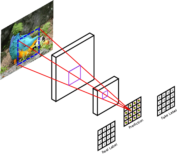
Overview

A GAN consists of two models

the Generator \(G_{\theta}\) which takes a vector of random noise \(z \sim p_{noise}(\cdot)\) as input and tries to generate a realistic image \(x = G_{\theta}(z)\) to images to fool the discriminator into thinking they are real
the Discriminator \(D_{\phi}\) which is a classifier which takes in an image \(x \sim p_{data}(\cdot)\)and identify the real images from the fake, outputting \(D(x) = 1\) for real images and \(D(x) = 0\) for fake images.

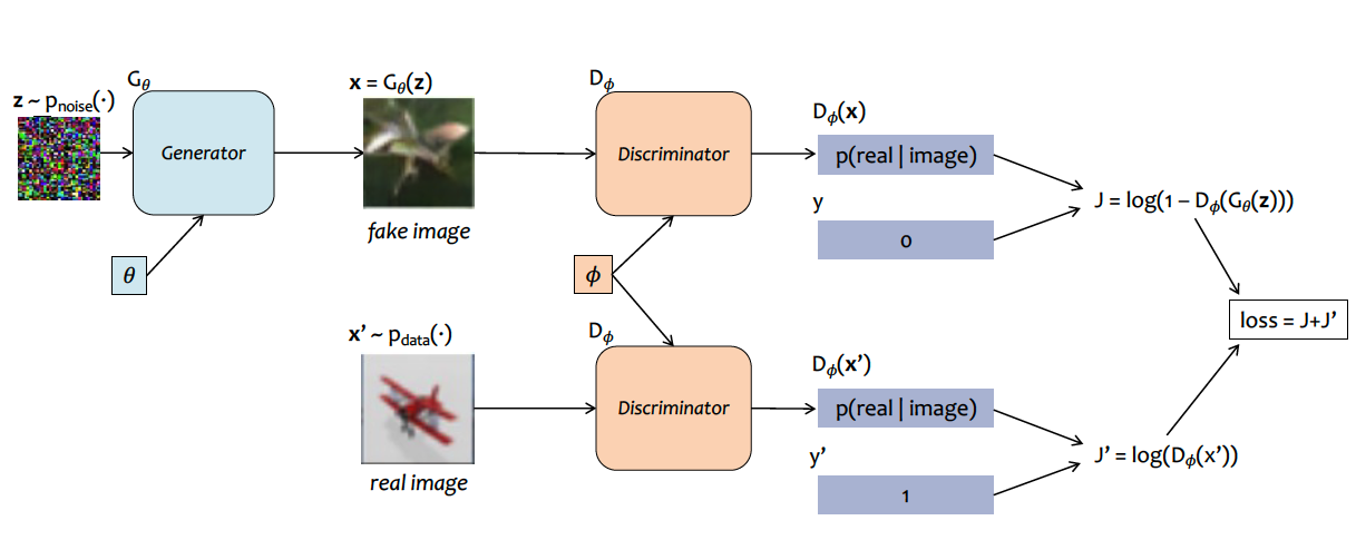
The Generator is the goal and the only item necessary for generating images during inference, but we need to train a Generator with the Discriminator which have opposite, Adversarial training objectives.

Loss Formulation

Goal

For the discriminator

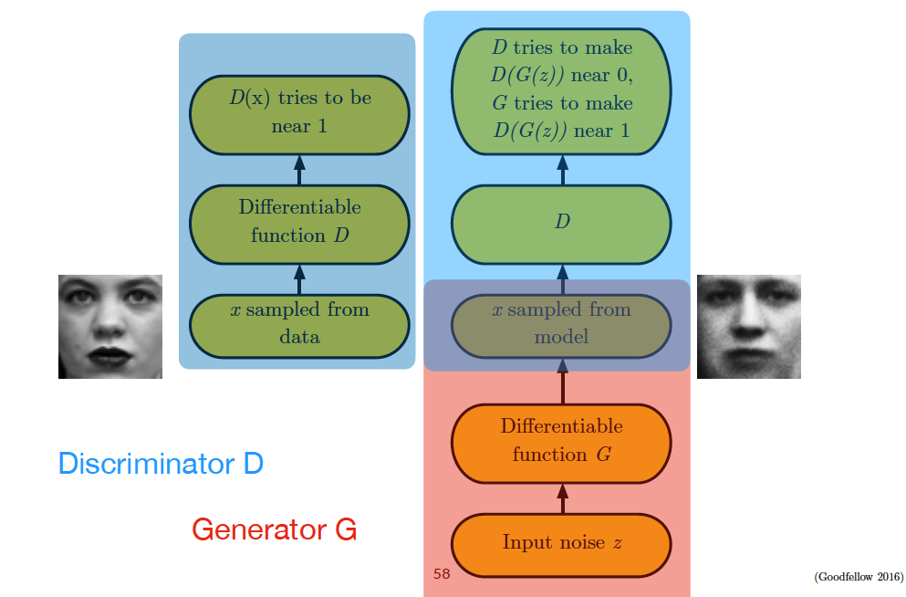
For real data \(x'\) we aim to maximize \(\log(D_{\phi}(x'))\) - we want \(D_{\phi}(x')\) to be 1
For synthetic data \(x\) we aim to maximize \(\log(1 - D_{\phi}(x))\) - in other words we want \(D_{\phi}(G_{\theta}(z)) = 0\)

For the generator

we want to trick the discriminator into believing that our generated synthetic data is real or equivalently minimize the likelihood that its generated image is classified as fake we aim to minimize \(\log(1- D_{\phi}(x))\) or we want \(D_{\phi}(G_{\theta}(z))=1\)

Formula

This leads to the following min-max optimization as our loss!

\[{\color{red}\min_{\theta}} \; {\color{blue}\max_{\phi}} \; J(\theta, \phi)= \underbrace{\mathbb{E}_{x'}\!\left[\log {\color{blue} D_{\phi}(x')}\right]}_{\text{real samples}} + \underbrace{\mathbb{E}_{z}\!\left[\log\!\left(1 - {\color{blue} D_{\phi}}\!\left({\color{red} G_{\theta}(z)}\right)\right)\right]}_{\text{fake samples}}\]

Inner \(\max_{D_{\phi}}\) discriminator’s problem

maximize 1st term: for actual data reward \(D\) for modeling high probability on real samples
maximize 2nd term: reward \(D\) for outputting low probability on fake examples

Outer \(\min_{G_{\theta}}\) generator’s problem

1st term does not depend on \(G\), because generator never sees real samples (so its vacuously true that we are trying to minimize the first term)
minimize 2nd term so that the log term becomes as negative as possible, clashing with the discriminator.

Interpreting the GAN Objective

Suppose we trained the discriminator and generator to an equilibrium where there generated samples where indistinguishable.

What does it mean if the discriminator were perfect for the current generator, then what objective is the generator actually optimizing?

A Bayes-optimal classifier is the classifier that makes the best possible decision if you knew the true optimal probabilities; in this case given the true data densities and the generator densities, the best possible discriminator (binary classification) determining the probability that a image sample came from real data rather than the generator would be:

\[D_{\phi}^*(x) = \frac{p_{data}(x)}{p_{data}(x) + p_{G_{\theta}}(x)}\]

Where \(p_{G_{\theta}}(x)\) denotes the distribution induced by sampling \(z \sim p_{noise}(\cdot)\). This minimizes the error rate in this equilibrium situation. Then if we substituted this optimal discriminator into our GAN objective yields

\[\begin{align*} J(\theta, \phi^*) &= \mathbb{E}_{x' \sim p_{data}(\cdot)}[\log D_{\phi}^*(x')] + \mathbb{E}_{z \sim p_{noise}(\cdot)}[\log(1 - D_{\phi}^*(G_{\theta}(z)))] \\ &= \mathbb{E}_{x \sim p_{data}(\cdot)} \left[ \log \frac{p_{data}(x)}{2\left(\frac{p_{data}(x)+p_{G_{\theta}}(x)}{2}\right)} \right] + \mathbb{E}_{x \sim p_{G_{\theta}}(\cdot)} \left[ \log \frac{p_{G_{\theta}}(x)}{2\left(\frac{p_{data}(x)+p_{G_{\theta}}(x)}{2}\right)} \right] \\ &= \mathbb{E}_{x \sim p_{data}(\cdot)} \left[ \log \frac{p_{data}(x)}{\frac{p_{data}(x)+p_{G_{\theta}}(x)}{2}} \right] + \mathbb{E}_{x \sim p_{G_{\theta}}(\cdot)} \left[ \log \frac{p_{G_{\theta}}(x)}{\frac{p_{data}(x)+p_{G_{\theta}}(x)}{2}} \right] - \log 4 \\ &= \mathrm{KL}\!\left(p_{data} \,\middle\|\, \frac{p_{data}+p_{G_{\theta}}}{2}\right) + \mathrm{KL}\!\left(p_{G_{\theta}} \,\middle\|\, \frac{p_{data}+p_{G_{\theta}}}{2}\right) - \log 4 \\ &= 2\,\mathrm{JSD}(p_{data} \parallel p_{G_{\theta}}) - \log 4 \end{align*}\]

What the GAN is doing is minimizing the JSD - Jensen-Shannon Divergence between the real distribution and the synthetic data distribution, trying to make the distributions maximally similar, which at ideal equilibrium means that

\[p_{G_{\theta}}(x)=p_{data}(x) \implies D_{\phi}^*(x) = \frac{p_{data}(x)}{p_{data}(x) + p_{G_{\theta}}(x)} = \frac{1}{2}\]

In ideal equilibrium, the derivative \(\mathrm{JSD}(p_{data} \,\|\, p_{G_{\theta}}) = 0\) since the distributions are the same, so the loss \(L\) is minimal and gradient for \(\phi, \theta\) is zero, completing training.

Now, the discriminator is not used after training to convergence, and the generator is used to generate data.

Iterative Training

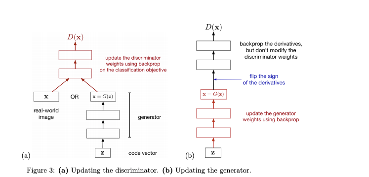
Using SGD-like algorithm of choice

Optimize on a minibatch of training examples the discriminator training objective for \(k\) steps In general, the discriminator must be trained first and must be updated more frequently, since the loss is what guides the training of the generator!
Optimize on a minibatch of generated samples the generator training objective for \(k\) steps

GAN training is unstable because this iterative game needs to be stable

if the discriminator gets too strong (nearly perfect) over on, then the gradient signal for the generator is too small for it to improve
if the generator is able to exploit a weakness in the discriminator, it may learn a narrow set of outputs leading to mode collapse

Shortcomings of Vanilla GAN

1. Vanishing Gradients

What if we train the discriminator till convergence (it is just a supervised classifier…) and becomes perfect in distinguishing real from generated images? If the discriminator is trained very well already, then it becomes very good at discriminating the fake images produced by the generator:

\[D(G(z)) \approx 0\]

which means the gradients are not very informative because \(\log(1 - D(G(z))) \approx \log (1 - 0) = 0\), giving no helpful learning signal.

Non-Saturated Generator Loss

Instead we can actually rewrite the original learning objective for the discriminator in terms of minimization:

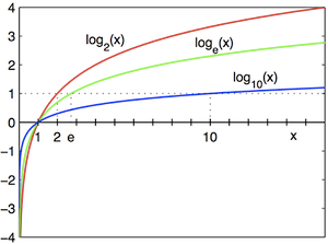
\[\max_D \mathbb{E}_{x\sim p_{data}}[\log D(x)] + \mathbb{E}_{z\sim p_z}[\log(1 - D(G(z)))] = \min_{D} \mathbb{E}_{x \sim p_{data}}[\log (1 - D(x))] + \mathbb{E}_{z \sim p_{z}}[\log D(G(z))]\]

Now the \(\log D(G(z))\) term actually gives a much more informative slope when \(D(G(z))\) is small:

The slopes between y=0 and y=1 are very different for different log-based objectives

2. Mode Collapse

Note that JSD - Jensen-Shannon Divergence is not our true training process. We alternate training the discriminator and generator which can lead to mode collapse, which happens when the generator always collapses to a small set of samples. For different \(z\), the generator produces similar output.

If \(G\) finds a small set of outputs that heavily fool \(D\), it can get a good average loss even though it completely ignores other modes.

Earth-Mover Distance or Wasserstein Distance

Think of transporting masses from one point to the other, implies there is an optimal use the least work to transport different masses to other point to make two piles of earth mass identical!

With Wasserstein Distance, if the generator distribution \(p_{G_{\theta}}\)has high peaks in the modes it chooses, while the true data \(p_{data}\) is much more spread, this measurement gives informative signal to spread probability mass across all modes .

Variants of GANs

DCGAN

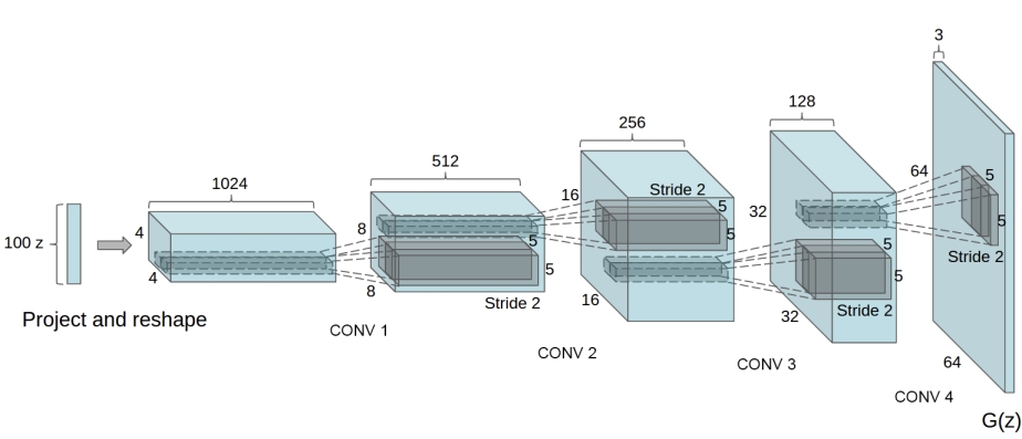
Here is generator: an inverted CNN with four fractionally strided convolution layers growing the size of the image from layer to layer.

PatchGAN

A PatchGAN discriminator uses a CNN to look at each patch of the image and predict whether its real or fake. We consider a receptive field of \(N \times N\) patches. The loss will aggregate a loss over each patch when determining the real or fake prediction.