Still in-progress writing

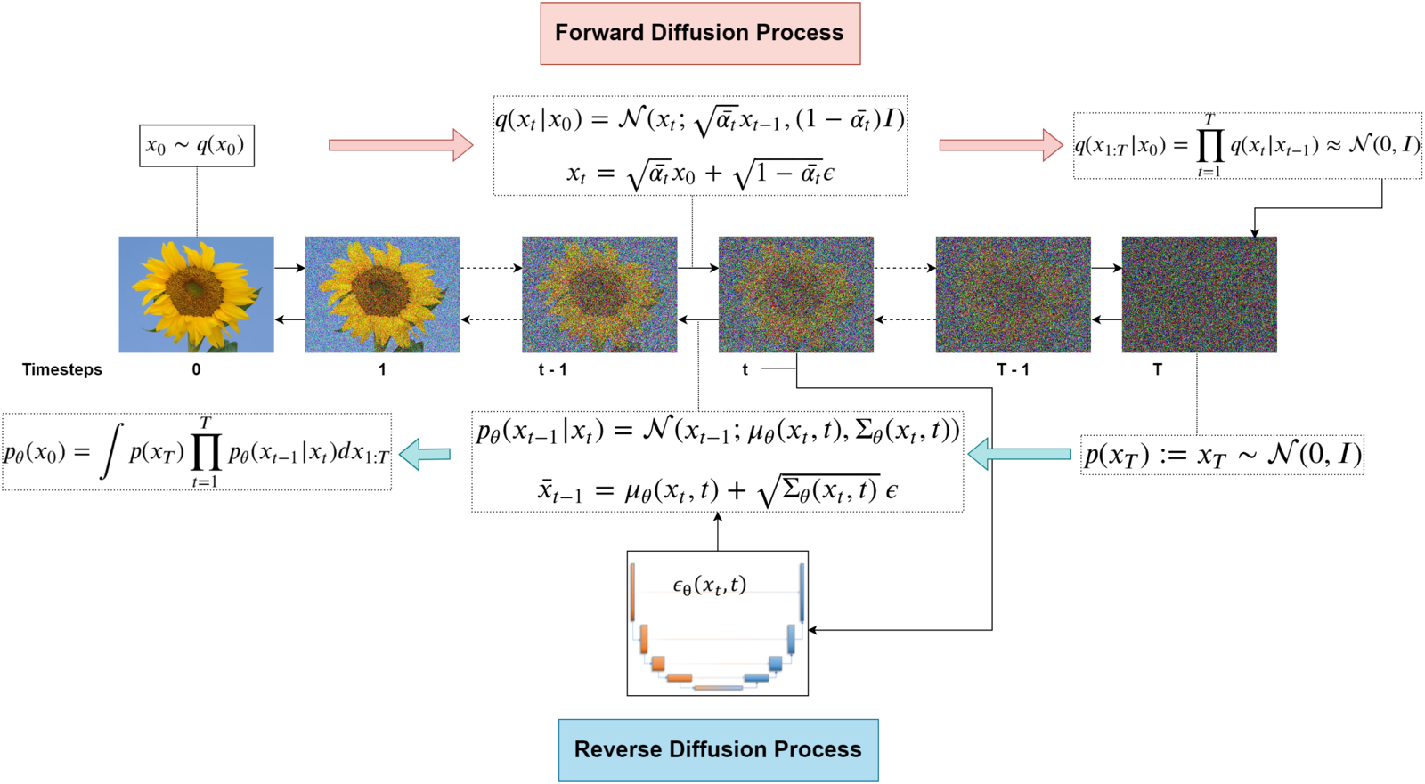
Forward Diffusion Process

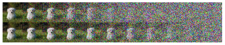
Given an image data point $x_{0}$ sampled from the image dataset distribution $x_{0} \sim q (x)$ , let us gradually add Gaussian Noise in a series of $T$ time steps, producing a sequence of noisy images ( $x_{1}, \dots x_{T}$ ) where $x_{i}$ is the image after the first $i$ steps.

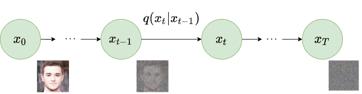
More formally this process can be described as the following: our image of $d$ pixels can be flattened to a vector $\in R^{d}$ and for type-checking purposes can be normalized into pixel intensities $[- 1, 1]$ (instead of $[0, 255]$ ). Each transition step is a conditional probability distribution ( $q (x_{t} ∣ x_{t - 1}) : R^{d} \to R^{+}$ ), giving us the probability density for the image $x_{t}$ given the previous time step’s $x_{t - 1}$ . We call this process Markovian, because it satisfies the Markov Property: each step only relies on the previous step (more formally $q (x_{t} ∣ x_{0 : t - 1}) = q (x_{t} ∣ x_{t - 1})$ )

x_{t} \sim q (x_{t} ∣ x_{t - 1}) = N (x_{t}; μ_{t} = \sqrt{1 - β_{t}} x_{t - 1}, Σ_{t} = β_{t} I)

To clarify some notation:

Retrieving image $x_{t}$ means retrieving from a Gaussian distribution denoted by $N (mean, variance)$

Mean: $μ_{t} = \sqrt{1 - β_{t}} x_{t - 1}$ of each pixel

Covariance: $Σ_{t} = β_{t} I$ (where $I = R^{d \times d}$ is the identity matrix)

What this means is that each individual pixel (with variance at $Σ_{p, p} = β_{t}$ ) is independently distributed of each other since off-diagonal entries $Σ_{p, q} = 0$ .

Using the reparameterization trick from VAEs, this means $x = μ + σ ⊙ ϵ, ϵ \sim N (0, I), (ϵ \in R^{d})$

$β_{t} \in [0, 1]$ is a constant given from our noise scheduler, $(β_{1}, β_{2}, \dots, β_{T})$ specifying the variance (noise intensity) added each time step. One interesting question one might have is why include the $\sqrt{1 - β_{t}}$ coefficient for mean. According to the reparameterization trick, since $x_{t} = \sqrt{1 - β_{t}} x_{t - 1} + \sqrt{β_{t}} ϵ$ , and because $x_{t - 1}$ and $ϵ$ are sampled from independent gaussians we can state

v a r (x_{t}) = v a r (\sqrt{1 - β_{t}} x_{t - 1}) + v a r (\sqrt{β_{t}} ϵ) = (1 - β_{t}) v a r (x_{t - 1}) + β_{t} \cdot 1

Since we normalized our image to $[- 1, 1]$ , $v a r (x_{0}) \leq 1$ , so then $\forall t, v a r (x_{t}) \leq 1$ . Apparently, this is called “variance preserving”. If our input $v a r (x_{0}) \approx 1$ , then $v a r (x_{t}) \approx 1$ as well. The point is the variance is constant through the entire forward process!

Variance/Noise Schedule

Originally, the authors of DDPM utilizes a linear schedule.

Variance Schedule of Linear (top) vs Cosine (bottom)

Simplified Sampling Form

The joint distribution of the entire trajectory of $T$ time steps, the product of all $T$ different PDF —

\begin{aligned} (Chain rule) & q (x_{1 : T} ∣ x_{0}) & = \prod_{t = 1}^{T} q (x_{t} ∣ x_{0 : t - 1}) \\ (Markov Property) & = \prod_{t = 1}^{T} q (x_{t} ∣ x_{t - 1}) \end{aligned}

— can be expressed a simpler closed form expression if we define a additional variables

$α_{t} = 1 - β_{t}, t = 1, \dots, T$ defining “fraction” of the previous step’s signal retained
${\bar{α}}_{t} = \prod_{s = 1}^{t} α_{s}$ denoting the fraction of the original image left after $t$ time steps.
$ϵ_{0}, \dots, ϵ_{t - 1} \sim N (0, I), ϵ_{i} \in R^{d}$ is the gaussian noise added at each time step and induct on $t$ or $x_{t}$ :

\begin{aligned} (Base Case) & x_{1} & = \sqrt{α_{1}} x_{0} + \sqrt{1 - α_{1}} ϵ_{0} = \sqrt{{\bar{α}}_{1}} x_{0} + \sqrt{1 - {\bar{α}}_{1}} ϵ_{0} \\ \dots \\ (Inductive Case) & x_{t} & = \sqrt{α_{t}} x_{t - 1} + \sqrt{1 - α_{t}} ϵ_{t - 1} \\ (Inductive Hypothesis) & = \sqrt{α_{t}} (\sqrt{{\bar{α}}_{t - 1}} x_{0} + \sqrt{1 - {\bar{α}}_{t - 1}} ϵ^{'}) + \sqrt{1 - α_{t}} ϵ_{t - 1} \\ = \sqrt{α_{t} {\bar{α}}_{t - 1}} x_{0} + \sqrt{α_{t} (1 - {\bar{α}}_{t - 1})} ϵ^{'} + \sqrt{1 - α_{t}} ϵ_{t - 1} \\ (Combine Variance Step) & = \sqrt{{\bar{α}}_{t}} x_{0} + [\sqrt{α_{t} (1 - {\bar{α}}_{t - 1})} ϵ^{'} + \sqrt{1 - α_{t}} ϵ_{t - 1}] \\ (See below) & = \sqrt{{\bar{α}}_{t}} x_{0} + \sqrt{1 - {\bar{α}}_{t} ϵ} \end{aligned}

The key combined variance step is as follows: Since $ϵ_{t - 2}$ and $ϵ_{t - 1}$ are sampled independently, the linear combination of independent Gaussians stays Gaussian, and yields a merged standard deviation as follows

v a r (X + Y) = v a r (X) + v a r (Y) + 2 c o v (X, Y) = α_{t} (1 - {\bar{α}}_{t - 1}) I + (1 - α_{t}) I = (1 - α_{t} {\bar{α}}_{t - 1}) I = (1 - {\bar{α}}_{t}) I

which allows us to replace $ϵ^{'}, ϵ_{t - 1}$ as sampling from a shared $ϵ \sim N (0, I)$ Thus we can write

x_{t} = \sqrt{{\bar{α}}_{t}} x_{0} + \sqrt{1 - {\bar{α}}_{t}} ϵ

and thus produce a sample

x_{t} \sim q (x_{t} ∣ x_{0}) = N (x_{t}; \underset{mean}{\underset{⏟}{\sqrt{{\bar{α}}_{t}} x_{0}}}, \underset{covariance}{\underset{⏟}{(1 - {\bar{α}}_{t}) I}})

As $T \to \infty$ , then we should have reached an isotropic Gaussian distribution, one where $x_{T} \sim N (0, I)$ follows a perfect gaussian distribution of mean $0$ . Note that is because ${\bar{α}}_{t} \to 0$ !

This is advantageous, because we all already know how to sample gaussian noise, so figuring out how to reverse the gaussian noise in the reverse diffusion process allows us to generate random images!

Reverse Diffusion Process

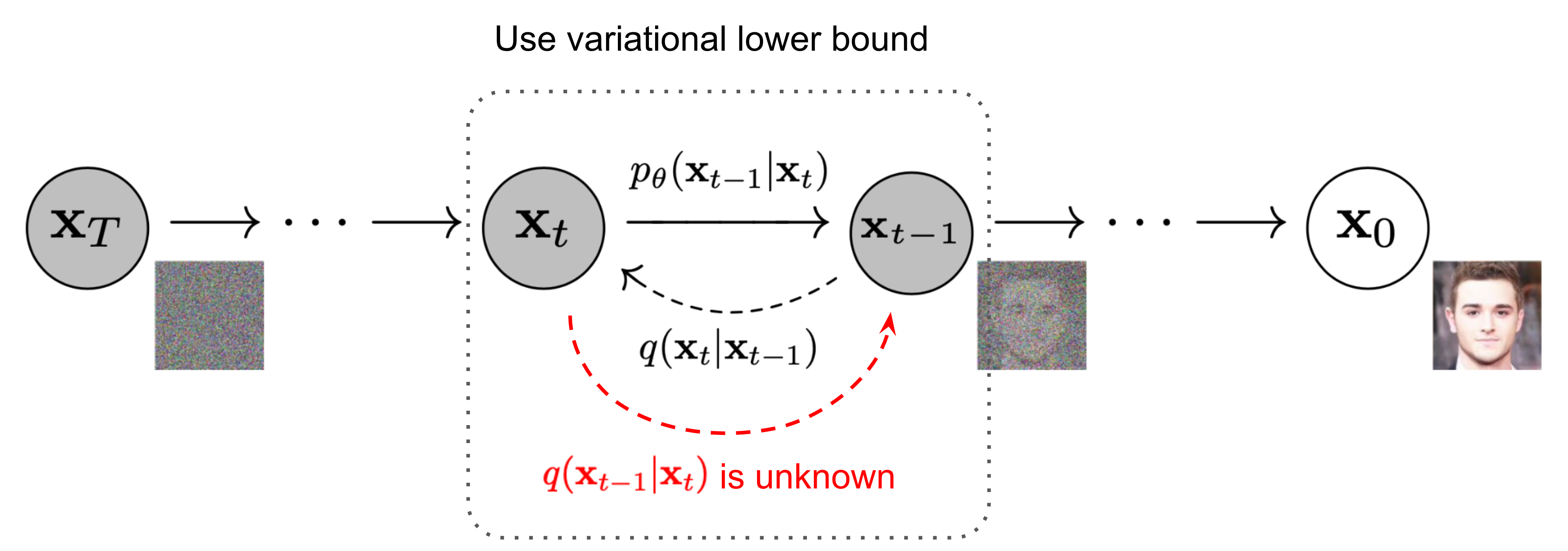
We want to learn the reverse distribution $q (x_{t - 1} ∣ x_{t})$ to acquire some new images in our dataset $x_{0}$ by learning a deep learning model by $p_{θ}$ where we learn some estimate mean and variance through parameters $θ$ :

p_{θ} (x_{t - 1} ∣ x_{t}) = N (x_{t - 1}; μ_{θ} (x_{t}, t), Σ_{θ} (x_{t}, t))

One specific path we may take from $x_{T} \to x_{0}$ is represented by

p_{θ} (x_{0 : T}) = p (x_{T}) \prod_{t = 1}^{T} p_{θ} (x_{t - 1} ∣ x_{t})

But the PDF of the entire reverse diffusion process is an “integral” over all the possible pathways we can take to reach $x_{0}$ .

p_{θ} (x_{0}) = \int p_{θ} (x_{0 : T}) d x_{1 : T}

DDPM - Denoising Diffusion Probabilistic Models

Forward Diffusion Process

Variance/Noise Schedule

Simplified Sampling Form

Reverse Diffusion Process

Classifier-Free Guidance

Latent DDPM

Stable Diffusion

Sources